Summary

Activation functions are crucial in neural networks, introducing non-linearity and enabling the modeling of complex patterns across varied tasks. This guide delves into the evolution, characteristics, and applications of state-of-the-art activation functions, illustrating their role in enhancing neural network performance. It discusses the transition from classic functions like sigmoid and tanh to advanced ones such as ReLU and its variants, addressing challenges like the vanishing gradient problem and the dying ReLU issue. Concluding with practical heuristics for selecting activation functions, the article emphasizes the importance of considering network architecture and task specifics, highlighting the rich diversity of activation functions available for optimizing neural network designs.

Introduction

In the fascinating world of neural networks, activation functions play a pivotal role. They introduce non-linearity into an otherwise linear model, enabling neural networks to learn complex patterns and solve a wide range of tasks. In this article, we will explore the state-of-the-art activation functions, diving into their history, characteristics, and trade-offs. By the end of this comprehensive guide, you will have a clearer understanding of when to employ each activation function to get better results from your network. Sources and related papers are listed throughout the guide, and I’d recommend reading them to know more about those activation functions. Towards the end, some heuristics are also provided for chosing activation functions.

Understanding Activation Functions

As a refresher, let’s establish an understanding of what activation functions are and why they are essential. During a forward pass of a neural network, at each neuron, the weighted sum of its inputs is calculated, along with the bias. This sum is called the preactivation value at that neuron.

Note: For this guide, we’ll focus on functions that operate on the scalar preactivations at each neuron individually. This approach is adopted because majority of the research and practical applications center around these types of activation functions. Activations like softmax and maxout that operate on an entire layer rather than a single neuron, are not covered.

Activation functions are fixed functions applied to the preactivation value at each neuron to get that neuron’s output. Mathematically, activation function is any real valued function Φ: ℝ → ℝ such that the neuron’s output is Φ(z), where z is the preactivation value. Additionally, activation functions need to be numerically differentiable (or made differentiable at kinks, eg. for ReLU) so that the weights can be updated during backpropagation. The primary purpose of Φ(z) is to introduce non-linearity, enabling neural networks to model complex relationships in data. Without activation functions, neural networks would reduce to linear models, incapable of handling intricate tasks such as image recognition, natural language processing, and more.

The Classic Choices

The evolution of activation functions has been instrumental in the progress of neural networks.

Cybenko (1989) and Hornik et al. (1989) showed that a feed-forward neural network with a single hidden layer (with sufficiently large number of neurons) can arbitrarily approximate any continuous real valued function (on a compact subset), given that the activation functions are non-constant, monotonically-increasing and bounded functions. — Apicella (2021)

These results are commonly referred to as the Universal approximation theorems, and they led to the popularization of two classic activation functions. Historically, sigmoid and tanh functions dominated the activation function landscape, as they satisfied the boundedness and monotonically-increasing conditions required for the above results. Let’s look at these two functions first.

1. Logistic function

The logistic activation function (commonly referred as just the sigmoid function, sigmoid functions are mathematical functions with a S-shaped curve) is defined as

Graphically, the logistic function is an S-shaped bounded and monotonically-increasing curve as shown below. Note how this satisfies the conditions required by the Universal approximation theorem.

Pros

• Smooth, differentiable, and interpretable function
• Outputs are between 0 and 1, making it suitable for binary classification.

Cons

• Prone to the vanishing gradient problem, hindering training in deep networks. This was shown in Benjio et al. (1994) and Hochreiter (1998) in the context of training Recurrent neural networks (trained as deep feedforward networks with shared weights). As can be observed from the logistic function graph, the derivative approaches close to zero for most of the input domain (|z| >5). In deeper networks, when the gradients get multiplied per the chain rule while performing backpropagation, the gradient vanishes exponentially for most of the input domain. As a result of these vanishing gradients, the weights close to input layers stop getting updated. You can read more in Benjio et al. (1994), Hochreiter (1998) and Wiki.
• Outputs are not zero-centered, causing slower convergence in certain situations. Having positive outputs from the logistic activation feed into the next layer means that the gradients w.r.t. the next layer’s weights would all have the same sign. As a result, the optimizer has to zigzag its way to the optima if the direction is not aligned with the gradient. More details are discussed in LeCun et al. (2012) Section 1.4.3 and 1.4.4.

2. Hyperbolic Tangent (tanh)

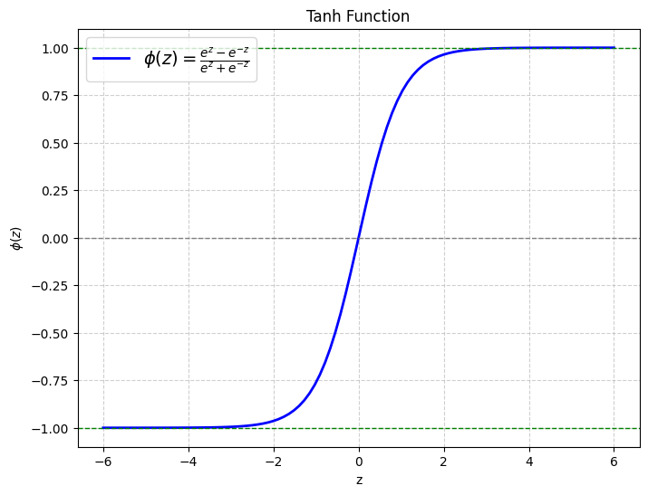
Another classic function that satisfies the conditions for the Universal Approximation theorems is the tanh function defined as:

The graph of tanh function is similar to the logistic function, but note that the output is zero-centered. This is one of the reasons that tanh is almost always preferred as an activation function over the logistic function, because the zero-centered outputs facilitate faster convergence as discussed before.

However, tanh activation still suffers from the vanishing gradient problem because the derivative approaches 0 for mildly small values of |z|.

The ReLU family

Pinkus (1999) proved that the boundedness requirement for activation functions in the Universal approximation results was unnecesarrily restrictive. Pinkus showed that the universal approximation property held even if the activation functions were unbounded, but not polynomial. Removing the boundedness constraint meant that activation functions no longer needed to suffer from vanishing gradients. Now, let’s explore some of the state-of-the-art activation functions that have emerged in recent years, addressing the limitations of their predecessors.

1. Rectified Linear Unit (ReLU)

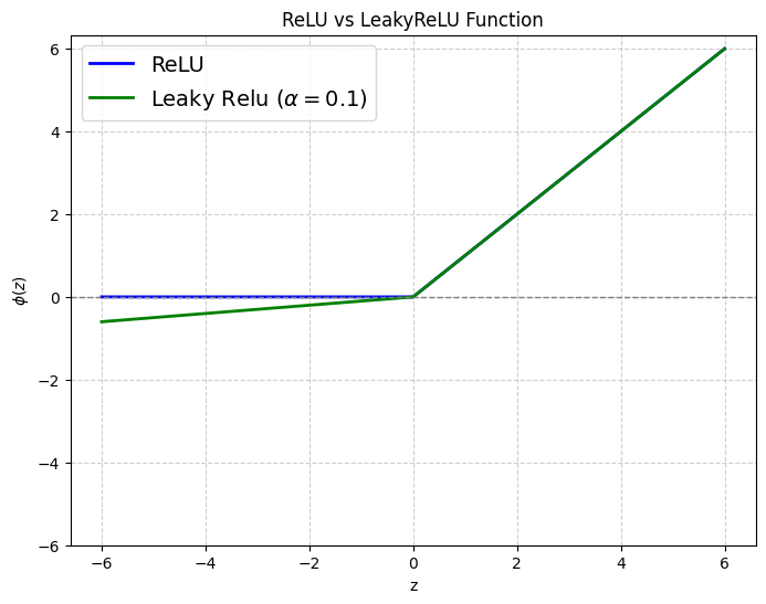
ReLU, one of the simplest activation functions (ignoring the identity activation) is defined as:

First used by Fukushima (1975), ReLU was repopularized by Nair & Hinton (2010) and the success of Glorot et al. (2011) and AlexNet (2012) in the 2010s cemented it as the primary activation function of choice for deep networks. The simple definition (the absence of exponentials) makes ReLU fast to compute and differentiate while training neural networks. Note however that ReLU is not differentiable at z = 0, as the left derivative is 0, while the right derivative is 1. In practise, a preactivation equal to 0 is rare, but floating point precision makes it not-so-rare. One can use any subgradient while performing optimizations. Popular choices are setting Φ’(0) = 0 (autograd libraries like PyTorch, Tensorflow do this) to favor sparcity in the feature maps, 0.5 and 1. The figure below shows the plot of the ReLU function:

ReLU has a following added advantage of inducing sparsity:

“The rectifier activation function allows a network to easily obtain sparse representations. For example, after uniform initialization of the weights, around 50% of hidden units continuous output values are real zeros, and this fraction can easily increase with sparsity-inducing regularization” — Glorot et al. (2011)

Sparse representations lead to better information disentanglement (by encouraging model simplicity), tend to be more robust to small changes in the input, and can be more interpretable than denser networks [Glorot et al. (2011)]. In addition, sparse representations have a smaller memory footprint (making them better for mobile devices) and have faster training times [Hoefler et al. (2021)].

ReLU also alleviates the vanishing gradient problem as it has a constant gradient of 1 for positive inputs. It might seem that having a gradient of 0 for z < 0 would be problematic. Glorot et al. (2011) answers this:

“One may hypothesize that the hard saturation at 0 may hurt optimization by blocking gradient back-propagation. […] However, experimental results (see Section 4.1) tend to contradict that hypothesis, suggesting that hard zeros can actually help supervised training. We hypothesize that the hard non-linearities do not hurt so long as the gradient can propagate along some paths, i.e., that some of the hidden units in each layer are non-zero. With the credit and blame assigned to these ON units rather than distributed more evenly, we hypothesize that optimization is easier.”

ReLU however suffers from the aptly-named “dying ReLU” problem, where some of the neurons (up to 50% dead neurons can be seen in practise) can become inactive during training. This can happen when a gradient update during backpropagation makes the bias of that neuron a large negative value. Then, for any data point chosen in the following iterations, the preactivation of that neuron would be negative, and it would always output 0 and backpropagate 0 gradients, effectively being dead. Note that even when some of the data points can make the preactivation > 0, the neuron is not dead and can learn gradually over iterations. High learning rates can also manifest as the dying ReLU problem, because a small gradient update can be magnified by the high learning rate, updating the bias term to a large negative value.

2. Leaky Rectified Linear Unit (Leaky ReLU)

Leaky ReLU is a variant of the ReLU function that allows small negative values, mitigating the dying ReLU problem by allowing small gradients for negative preactivations.

The parameter α controls the slope for negative values and is generally chosen to be a small value in the range [0, 1]. A default choice of α is 0.01 in various libraries.

By allowing negative values, LeakyReLU can also have faster convergence since the mean of outputs shifts towards 0. The performance of the network with leaky ReLU depends on the parameter α, which must be carefully chosen or the performance can be worse than with ReLU activations. Given its efficacy, LeakyReLU is widely used in Convolutional Neural Networks (CNNs) like the YOLO object detection model and in Generative Adversarial Networks (GANs) like DCGAN.

3. Parametric Rectified Linear Unit (PReLU)

PReLU proposed in He et al. (2015) turns the slope parameter in Leaky ReLU into a trainable parameter aᵢ, i being the channel number of the CNN used in the original paper. In practise, different strategies can be employed to either share the param aᵢ among neurons in a layer or across layers, depending on the compute power (since this increases the number of trainable parameters). While backpropagating, the parameter aᵢ gets updated as well. PReLUs can be used when it’s difficult to tune the parameter α with LeakyReLU activation functions, by letting the optimizer find the best slopes.

Related read: Xu, Bing, et al. “Empirical evaluation of rectified activations in convolutional network.” arXiv preprint arXiv:1505.00853 (2015).

4. Exponential Linear Unit (ELU)

As an improvement to ReLU, Clevert et al. (2015) proposed ELU defined as:

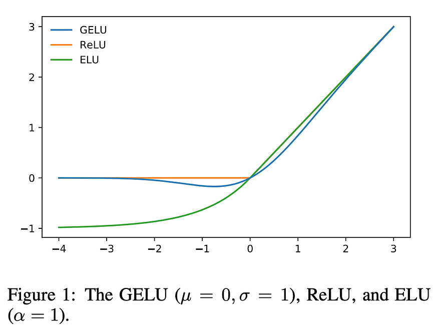
α is a hyperparameter here and can be tuned, a good starting point is α = 1. Like LeakyReLU and PReLU, exponential linear unit also has non-zero outputs for z < 0. In contrast to the other two alternatives, ELU output saturates to a negative output for large negative input values (shown in the graph below). This allows ELU to learn a more robust representation while preventing the dying ReLU problem.

“ELUs code the degree of presence of particular phenomena in the input, while they do not quantitatively model the degree of their absence.” — Clevert et al. (2015)

Since ELU is not piecewise linear, it has a better chance of modeling non-linearity. The slower computation time of ELU is compensated by its faster convergence rates when compared to ReLU, due to the mean of outputs being closer to 0. It has been shown to outperform ReLU and LeakyReLU on vision datasets like CIFAR-100 and ImageNet.

Related works:

1. Scaled Exponential Linear Units: Klambauer, Günter, et al. “Self-normalizing neural networks.” Advances in neural information processing systems 30 (2017).
2. Comparison with ReLU and LeakyReLU: Pedamonti, Dabal. “Comparison of non-linear activation functions for deep neural networks on MNIST classification task.” arXiv preprint arXiv:1804.02763 (2018).

Gaussian Error Linear Unit (GELU)

Hendrycks & Kevin (2016) proposed the GELU activation function modeled on a combination of properties of ReLU and dropout. Imagine a stochastic model where each input has a probability of being dropped (like dropout) but this probability depends on the input itself. This is the motivation behind this activation function, where the probability of being dropped is given by the cumulative distribution function (CDF)of the standard gaussian. The standard gaussian is chosen because batch normalization tends to produce inputs following the standard gaussian. Finally, to make the function deterministic, GELU’s output is the expected value of the ReLU function under this stochastic model:

Since this formulation is compute heavy, authors provide two approximations using tanh and the sigmoid function that can be used, depending on the desired speed vs exactness tradeoff. Following is a comparative graph of GELU, ReLU and ELU functions:

Note that the GELU curve is non-convex and not monotonically-increasing for z < 0. Also, GELU is smooth and differentiable at z = 0, which might be a reason for its faster convergence rate. It is hypothesized that this increased curvature and non-monotonicity allows GELU to better approximate more complicated functions than ReLU and ELU. GELU slightly outperforms both of the latter on MNIST autoencoding and CIFAR-10/100 classification. However, even GELU approximations are much slower than the simple ReLU or LeakyReLU functions. Due to its effectiveness, GELU is currently the SOTA for NLP tasks, and is used in models like BERT and OpenAI’s GPT series.

Swish

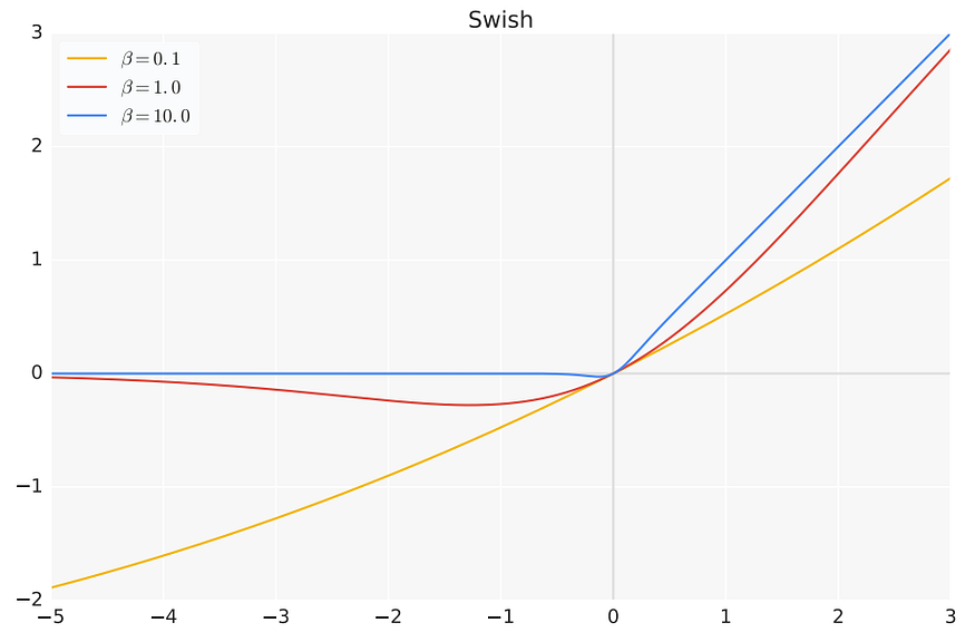
Ramachandran et al. (2017) set out to find novel activation functions using automated search techniques. The best discovered function according to their evaluations was named Swish, and is defined below:

Here β can be either a tuned constant or a trainable parameter for the model and σ is the standard logistic function. For β = 0, Swish is a linear function, while as β → ∞, Swish approaches the ReLU function (see figure below). So, it can be thought of as a smooth nonlinear interpolation between the linear and ReLU functions as one varies β. β = 1 is a good starting choice for the parameter.

Like GELU, Swish also has a non-monotonic bump close to origin, which could be a reason for its ability to model complex functions better than ReLU. Emperically, Swish is favoured over ReLU as the model gets deeper, and optimization becomes difficult. The authors show that Swish either outperforms or is at par with ReLU, PReLU and GELU on 9/9 tasks, and is beaten by ELU and LeakyReLU only on 1/9 tasks. These tasks vary from image classification on CIFAR and ImageNet datasets to machine translation. Like GELU, Swish also requires calculating the logistic function, which makes it computationally expensive compared to ReLU variants.

Conclusion

The choice of activation function is not one-size-fits-all. In this guide, we discussed classic activation functions and their drawbacks. Then we discussed the rise of ReLU and its improvements. Finally, we also looked at some lesser known state-of-the-art activations used in research as well as industry. Several factors influence your decision, including model size, the type of neural network architecture, and the nature of the task. Some rules of thumb are discussed below.

For shallow models, classic functions like sigmoid and tanh may perform reasonably well due to their smooth and bounded nature. Tanh is preferred over sigmoid due to its zero-centered outputs, leading to faster convergence. Depending on the type of task, these functions along with softmax (for multiclass classification) are good choices for the final layer activations.

In contrast, ReLU and its variants are often preferred for the hidden layers on large datasets and deeper models as they accelerate training. CNNs frequently benefit from the ReLU variants and the Swish activation function. When training a DNN, Leaky ReLU is generally a good starting point. Alternatively, one can chose ReLU activations and inspect the percentage of dead neurons, switching to LeakyReLU or PReLU if required. GeLU shines in NLP tasks despite its computational cost. Swish, while promising, is relatively new and requires further exploration, interpretability and testing.

The activation function landscape is rich and diverse, offering a spectrum of choices to cater to various neural network needs. I hope this guide served as a good starting point for more exploration based on your requirements and network design.

Featured Image created with Midjourney.

References

1. Cybenko, George. “Approximation by superpositions of a sigmoidal function.” Mathematics of control, signals and systems 2.4 (1989): 303–314.
2. Hornik, Kurt, Maxwell Stinchcombe, and Halbert White. “Multilayer feedforward networks are universal approximators.” Neural networks 2.5 (1989): 359–366.
3. Apicella, Andrea, et al. “A survey on modern trainable activation functions.” Neural Networks 138 (2021): 14–32.
4. Y. Bengio, P. Simard and P. Frasconi, “Learning long-term dependencies with gradient descent is difficult,” in IEEE Transactions on Neural Networks, vol. 5, no. 2, pp. 157–166, March 1994, doi: 10.1109/72.279181.
5. Hochreiter, Sepp. “The vanishing gradient problem during learning recurrent neural nets and problem solutions.” International Journal of Uncertainty, Fuzziness and Knowledge-Based Systems 6.02 (1998): 107–116.
6. LeCun, Y.A., Bottou, L., Orr, G.B., Müller, KR. (2012). Efficient BackProp. In: Montavon, G., Orr, G.B., Müller, KR. (eds) Neural Networks: Tricks of the Trade. Lecture Notes in Computer Science, vol 7700. Springer, Berlin, Heidelberg. https://doi.org/10.1007/978-3-642-35289-8_3
7. Pinkus, Allan. “Approximation Theory of the MLP Model in Neural Networks.” Acta Numerica, vol. 8, 1999, pp. 143–195., doi:10.1017/S0962492900002919.
8. Fukushima, K. Cognitron: A self-organizing multilayered neural network. Biol. Cybernetics 20, 121–136 (1975). https://doi.org/10.1007/BF00342633
9. Nair, Vinod, and Geoffrey E. Hinton. “Rectified linear units improve restricted boltzmann machines.” Proceedings of the 27th international conference on machine learning (ICML-10). 2010.
10. Glorot, Xavier, Antoine Bordes, and Yoshua Bengio. “Deep sparse rectifier neural networks.” Proceedings of the fourteenth international conference on artificial intelligence and statistics. JMLR Workshop and Conference Proceedings, 2011.
11. Krizhevsky, Alex, Ilya Sutskever, and Geoffrey E. Hinton. “Imagenet classification with deep convolutional neural networks.” Advances in neural information processing systems 25 (2012).
12. Hoefler, Torsten, et al. “Sparsity in deep learning: Pruning and growth for efficient inference and training in neural networks.” The Journal of Machine Learning Research 22.1 (2021): 10882–11005.
13. He, Kaiming, et al. “Delving deep into rectifiers: Surpassing human-level performance on imagenet classification.” Proceedings of the IEEE international conference on computer vision. 2015.
14. Clevert, Djork-Arné, Thomas Unterthiner, and Sepp Hochreiter. “Fast and accurate deep network learning by exponential linear units (elus).” arXiv preprint arXiv:1511.07289 (2015).
15. Hendrycks, Dan, and Kevin Gimpel. “Gaussian error linear units (gelus).” arXiv preprint arXiv:1606.08415 (2016).
16. Ramachandran, Prajit, Barret Zoph, and Quoc V. Le. “Searching for activation functions.” arXiv preprint arXiv:1710.05941 (2017).
17. https://www.v7labs.com/blog/neural-networks-activation-functions