Recent Posts

At 2100 UTC (5pm EDT) Friday, 25 October 2019, a well-defined but very small tropical storm with wind speeds of 45 mph formed in the Northeastern Atlantic Ocean. It formed within an occluded extratropical cyclone, which is the name of a late stage extratropical cyclone where the northern portion of the cold front “catches up” to the northern portion of the warm front within the cyclone. It is unusual, but not unheard of, for a tropical cyclone to form in such conditions. As can be seen in Fig. 1, the sea surface temperatures (SSTs) were around 23⁰C, outside of the normal 26.5⁰C or above SSTs typically needed to sustain a tropical cyclone. Due to the SSTs, the small size of the cyclone, and the baroclinic environment that resulted in the existence of the extratropical cyclone, the National Hurricane Center (NHC) forecasted that the then tropical storm Pablo would become extratropical within 36 hours or sooner. They also anticipated the tropical storm to slightly increase in wind speed. They did not, however, anticipate this small tropical storm would soon become a hurricane.

Figure 1: Sea Surface Temperatures on 26 October 2019. TS Pablo on 25 October is seen in blue labelled as “TS.” Hurricane Pablo on 27 October is seen in purple labelled as “H.” Source: NOAA

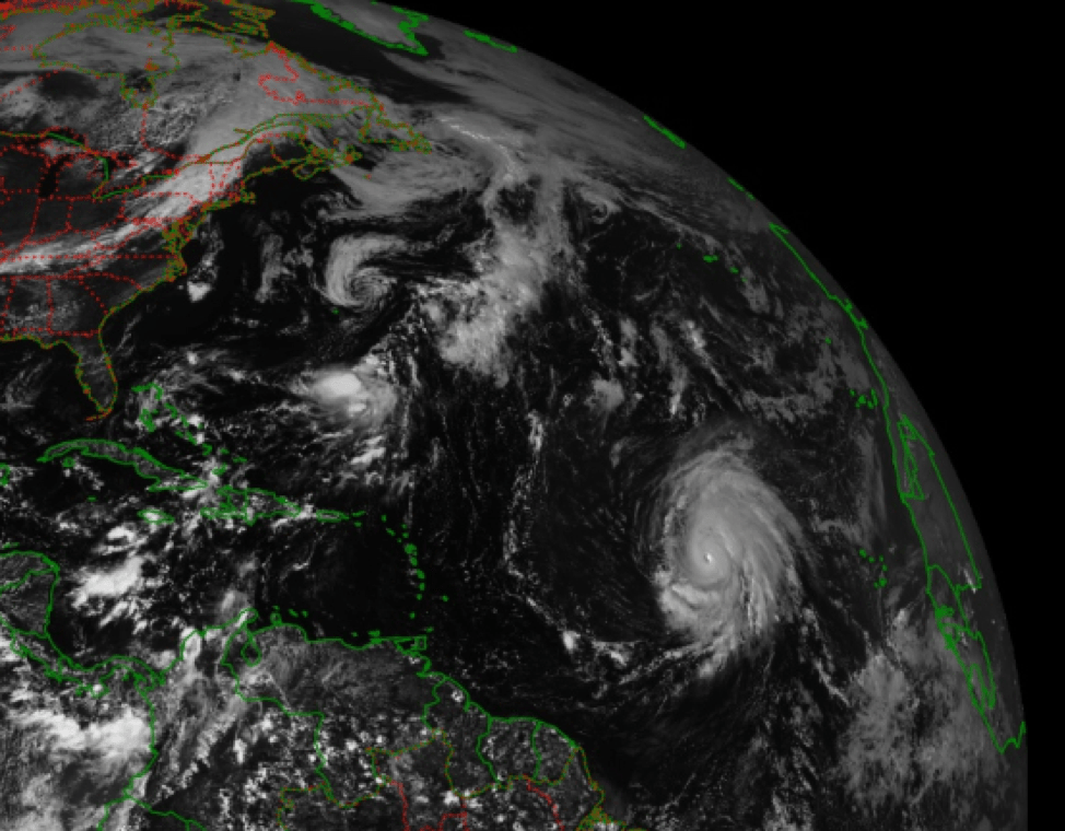
Over the next day, tropical storm Pablo strengthened unexpectedly to 60 mph and had formed an eye recognizable on satellite imagery, as seen in Fig. 2. While this came as a surprise, the tropical storm was heading towards colder waters and an environment of increased shear, both of which would result in the weakening of the storm. As a result, the forecasted transition to an extratropical cyclone remained, and tropical storm was expected to weaken.

Figure 2: IR Satellite image of TS Pablo at 1700 UTC (1pm EDT) on 26 October 2019. Source: EUMETSAT

However, tropical storm Pablo continued to defy expectations, strengthening into a category 1 hurricane with 80 mph winds at 2100 UTC (5pm EDT) on Sunday, 27 October 2019. This strengthening occurred despite SSTs of around 17⁰C (Fig. 1), and hurricane Pablo therefore became the furthest east and second furthest north storm on record to ever strengthen into a hurricane, as can be seen in Fig. 3. From there, over the course of the next 36 hours, hurricane Pablo weakened steadily, finally succumbing to the cold waters and increased shear. By 1500 UTC (11am EDT) on Monday, 28 October 2019, hurricane Pablo had weakened to a post-tropical cyclone.

Figure 3: Location of first intensification to a hurricane (1950-present). Source: Tomer Burg, Twitter

Sources:
https://www.washingtonpost.com/weather/2019/10/28/oddball-hurricane-pablo-developed-farther-east-than-any-atlantic-tropical-cyclone-record/
https://www.nhc.noaa.gov/archive/2019/PABLO.shtml
https://eumetview.eumetsat.int/mapviewer/

The National Weather Service has issued storm surge warnings and tropical storm warnings across the Gulf Coast in anticipation of the development of Tropical Storm Nestor. The system is currently an invest region in the center of the Gulf of Mexico. The system is expected to reach tropical storm force in the morning hours of 18 October, and will likely make landfall near Panama City, FL in the early morning hours on 19 October 2019. The system is forecasted to move quickly across the Southeast before making its way to the Atlantic, shown in Figure 1. It is not expected to reach hurricane status, but instead become a sub-tropical storm. This means the system will have characteristics of both a tropical storm and a regular storm system. The main threats are flooding and strong winds. Parts of the Gulf Coast could see up to six inches of rain and two to five feet of storm surge.

Figure 1. National Hurricane Center released forecasted storm track from 12Z 18 October 2019. The image depicts the location of the center of the system over the Gulf of Mexico, and the anticipated motion of the storm along the cone.

Figure 2. Both images taken from NESDIS GOES-16 satellite image viewer. Image on the left is a visible satellite image of the system at 1321Z 18 October 2019. Image on the right is an IR Cloudtop image taken at 1326Z 18 October 2019.

Using the satellite images above (Figure 2), we can get an idea of the relative size and strength of the system as it makes its way towards the coast. There is no defined eye, indicating that the system is not well organized. Systems with a defined eye typically have hurricane force winds and are stronger in nature. However, we can note that there is strong convection in the center of the system. The black and white color in the IR image indicates high level cloud tops, which is a characteristic of strong convection. This indicates the system is strengthening, which we would expect to see as it is over a body of warm water.

Sources:

https://www.weather.gov/

https://www.star.nesdis.noaa.gov/GOES/conus.php?sat=G16

Figure 1: One of eight microsatellites that comprise the Cyclone Global Navigation Satellite System (CYGNSS), which can be used for tropical cyclone research. (Source: NASA JPL)

While accurate forecasting of tropical cyclone intensity is inherently challenging, it is of high interest to society. Intensity predictions can be used to categorize a hurricane on the Saffir-Simpson Hurricane Wind Scale and prompt decision makers to issue storm warnings in a timely manner to protect lives and infrastructure. But with model biases, subjectivity, and limitations in analyses like the Dvorak Technique, Advanced Dvorak Technique, and ASCAT, how on Earth do meteorologists determine the intensity of a hurricane? Perhaps from space? (pun intended)

Microsatellites in low Earth orbit, which are only about the size of a microwave oven, offer an innovative and promising perspective for improving tropical cyclone intensity predictions. Researchers at NASA and the University of Michigan designed the Cyclone Global Navigation Satellite System, or CYGNSS. This eight microsatellite constellation, launched in December 2016, orbits the tropics at approximately 510km above the equator. Fig. 3 shows how the microsatellites deploy. Unlike traditional instruments such as the GOES Infrared Radiation and Visible products, CYGNSS detects reflected GPS signals which have L-band frequency. This long wavelength (~7.5 inches) is unobstructed by precipitation and atmospheric particles, meaning that CYGNSS can determine surface level sea roughness (which correlates to surface wind speeds) even within the most intense convection region of a hurricane: the eyewall. Surprisingly, CYGNSS is a passive satellite fleet. The GPS signal actually originates form GPS satellites in higher orbit, which are operated by the United States Air Force. Additionally, with an orbit period of only 95 minutes, each microsatellite passes within 12 minutes of the previous one. According to the mission’s Primary Investigator, Dr. Christopher Ruf, the data collected from CYGNSS is analogous to “a fleet of Hurricane Hunter airplanes distributed everywhere in the tropics.”

Figure 2: Comparison of tropical cyclone measurements from Advanced Dvorak Technique, CYGNSS, and a combination of products. When used in combination with other products, CYGNSS improves the overall model predictions. (Source: AGU Geophysical Research Letters)

In a paper published by AGU’s Geophysical Research Letters, when CYGNSS data from 2017 was combined with other tropical cyclone intensity prediction methods for hurricanes Irma and Harvey, the overall predictions improved. Fig. 2 shows wind speed and vector comparisons by the Advanced Dvorak Technique, CYGNSS, and a combination of methods, as well as surface latent heat flux. Since CYGNSS has only been in operation since 2017, researchers are still exploring and improving the applications of this small but mighty microsatellite fleet’s capabilities to improve tropical cyclone intensity forecasting.

Figure 3: Click the video to view how the eight microsatellites of CYGNSS deploy in low Earth orbit (Source: NASA)

Sources:

https://www.nasa.gov/feature/jpl/nasa-smallsats-can-aid-hurricane-forecasts-with-gps

https://agupubs.onlinelibrary.wiley.com/doi/full/10.1029/2019GL082236

https://podaac.jpl.nasa.gov/CYGNSS

https://www.nasa.gov/cygnss/overview

“Weather: A Concise Introduction” by Gregory Hakim and Jérôme Patoux

While the United States has had some tropical storm events happen closer to home, there’s now a formidable cyclone building in the mid-Atlantic, and its name is Lorenzo. On September 26, 2019, Lorenzo is classified as a category 3 hurricane, and expected to strengthen to category 4 in the near future. Fortunately for readers, Lorenzo is not expected to reach the United States as a hurricane, or any other landmass. Even if Lorenzo doesn’t make landfall, it is a great opportunity to observe hurricane formation unimpeded by landmasses. The eye is particularly striking in Figure 1, standing out from the cloud outflow surrounding it due to the angle of the Sun at the time of viewing.

Fig. 1. GOES-16 full disc visible imagery with Lorenzo west of the African coast, taken 26 September 2019 at 17:20 GMT (or 1:20 PM EDT).

Lorenzo is projected to become a category 4 hurricane, but it’s also likely to be demoted back to a category 3 soon after. Taking a look at the Airmass RGB data from GOES-16 and Meteosat may help answer why – green regions represents moist, tropical airmasses and rusty orange regions represent dry airmasses, and Lorenzo’s got a dry orange region similar in size to itself just to its west (Fig. 2). I’ve taken imagery from two satellites in this case because Airmass RGB tends to wrap the horizon with a blue/purple hue due to how it detects water vapor. If Lorenzo continues west, it will have to interact with the dry air region, which could weaken its development by halting moisture intake. If Lorenzo moves north, it will have to contend with cooler water temperatures that could also weaken its development, as colder seawater will evaporate less readily.

Fig. 2. GOES-16 (left) and Meteosat 0 degree (right) full disc Airmass RGB composite imagery of Lorenzo taken 26 September 2019 at 21:00 GMT (or 5 PM EDT).

The good news is that Lorenzo in its current form likely won’t directly impact continental landmasses. The bad news (for Lorenzo) is its possible trajectories all lead to a weakening system in the near future. Incidentally, the dry air region to Lorenzo’s west could be a fragment of the Saharan Air Layer, a hot and dry airmass that advects out of the Sahara during the warmer months. The SAL isn’t always loaded with dust, but it often is, and some dust particles on Dust RGB imagery can be seen to the west of Africa at the time of this post (Fig. 3). We could have Africa to thank for stopping Lorenzo from getting out of control!

Fig. 3. Meteosat 0 degree Dust RGB over Africa, taken 26 September 2019 at 18:00 GMT. Dust is represented in pink hues.

GOES-16 full disc visible imagery can be found at https://whirlwind.aos.wisc.edu/~wxp/goes16/vis/goes16_fulldisk.html

GOES-16 full disc Airmass RGB imagery can be found at https://whirlwind.aos.wisc.edu/~wxp/goes16/multi_air_mass_rgb/goes16_fulldisk.html

Meteosat full disc Airmass RGB imagery can be found at https://eumetview.eumetsat.int/static-images/MSG/RGB/AIRMASS/FULLDISC/index.htm

Meteosat full disc Dust RGB imagery can be found at https://eumetview.eumetsat.int/static-images/MSG/RGB/DUST/FULLRESOLUTION/

Figure 1: Map of age of recent lightning strikes in Texas on 19 September 2019 at 2110 UTC (map created through analysis of lightning detection sensors) (https://www.weathertap.com)

Cloud Height and Reflectivity Act as Maps of Lightning for Imelda

Imelda made landfall in Houston, TX as a tropical depression on Wednesday, 18 September 2019. It brought heavy precipitation and severe weather, including multiple tornado reports. Maps of lightning strikes associated with the storm within the hours before 2110 UTC 19 September 2019 display the effectiveness of using satellite imagery and radar imagery to identify areas of severe weather (Figure 1). The locations of lightning strikes within the 12-30 minutes prior to 2110 UTC (marked in white) display concentrations of lightning to the southwest, south, southeast, and northwest of Houston, as well as further north over Austin, TX. Satellite imagery of Texas within the IR Cloud Top channel display high clouds in the same areas, including significant cloud heights off the coast south of Galveston, TX, which may be too far from land to detect lightning strikes as there is not much recent lightning displayed in that location (Figure 2). Lightning is caused when deep convective clouds have large quantities of ice which aids in the polarization of the cloud structure. These ice particles result from water droplets high in the atmosphere freezing, but first they must reach altitudes cold enough. This is why deep clouds with significant heights are associated with lightning causing dynamics.

Figure 2: GOES-16 Infrared Cloud Top Imagery on 19 September 2019 at 2116 UTC (https://www.star.nesdis.noaa.gov/GOES/)

The base radar reflectivity is a less effective method of predicting the locations of large quantities of lightning strikes in the case of Imelda on 19 September 2019, with more areas of significant rainfall identified than had lightning strikes, such as to the north of Houston (Figure 3). The largest cell associated with the storm with respect to horizontal scale, just south of Houston and over Galveston, is easily apparent on the radar reflectivity image as a large area of reflectivity values over 40 Dbz.  It is less easy to identify cells further west that match up with the individual cells identifiable by the red colors indicating tall clouds on the satellite imagery. Radar also has the disadvantage of limited range and the fact that radar signals can be blocked from reaching regions on the opposite side of heavy precipitation from the radar. This indicates that in the case of Imelda, radar may have been unable to detect precipitation in regions with frequent lightning strikes; satellite imagery of cloud height acted as a fairly accurate map of regions with a high volume of lightning strikes.

Figure 3: Radar reflectivity map from KHGX (Houston, Tx) on 19 September 2019 at 2111 UTC (https://radar.weather.gov/ridge/radar.php?product=NCR&rid=HGX&loop=yes)

Late Tuesday night, on September 10^th, 2019, three tornadoes touched down and lifted over the course of five and a half minutes. All three were listed as an EF-2 on the Enhanced Fujita scale, and each tornado lasted roughly a minute. However, a tornado warning was not issued until two of the three tornadoes had already touched down and lifted, causing significant damage to the city of Sioux Falls. This delay in warning was due to the fact that tornadoes produced quasi-linear convective systems, or QLCS, are considerably harder to forecast than those formed in supercell thunderstorms.

Figure 1: Doppler radar (left) and storm relative velocity (right) of a supercell producing a tornado, Raleigh NC, April 16^th 2011. Source: USTornadoes.com

Unlike supercells (Figure 1), where the location and formation of these tornadoes can be more easily seen on radars with enough time to issue a warning, a QLCS can produce tornadoes with little to no warning. Some of these tornadoes can form in the time it takes the radar to complete a cycle the area, and disappear just as quickly. In Sioux Falls, they experienced just that. An initial scan with a storm relative velocity radar shows an area of developing circulation at 11:25pm (Figure 2, left), but was significant enough to send out a warning. One minute and 26 seconds later, the following scan at 11:26pm (Figure 2, right) indicated a tornado had already formed, and by the time the tornado warning was sent out another minute and 35 seconds later, a second tornado had touched down. Luckily, while the city suffered considerable property damage, no deaths or serious injuries have been reported due to this outbreak of tornadoes in Sioux Falls.

Figure 2: Storm Relative Velocity at 11:25pm (left) and 11:26pm (right), Sioux Falls, September 10^th 2019. Green indicated movement toward the radar site, while red indicates movement away from the radar site. Source: NOAA/GR2 Analyst/Matthew Cappucci

Sources:
https://www.washingtonpost.com/weather/2019/09/12/trio-tornadoes-tear-up-sioux-falls-sd/
https://www.ustornadoes.com/2013/02/14/understanding-basic-tornadic-radar-signatures/
https://www.washingtonpost.com/news/capital-weather-gang/wp/2017/04/20/americans-are-getting-less-advance-notice-for-tornadoes-as-researchers-struggle-to-understand-why/
https://www.usatoday.com/story/news/nation/2019/09/11/sioux-falls-south-dakota-tornado/2283760001/

Hurricane Dorian made history earlier this week as one of the most intense Atlantic basin hurricanes on record. In fact, it was the second strongest storm by wind speeds since 1950 in the Atlantic Basin. Dorian also made history as the strongest hurricane to make landfall in the Bahamas. The hurricane caused mass destruction to the Bahamas, striking the islands as a strong category 5 hurricane, and with winds peaking at 185 mph. The hurricane moved slowly over the region, contributing to major flooding on the islands. From 12am 2 September 2019 to 6am local time 3 September 2019, Dorian moved just 33 miles in 30 hours. A satellite image from ICEYE taken 2 September shows the extent of the flooding that occurred on Grand Bahama.

Grand Bahama satellite image depicting flooding. The yellow-green outline is the islands original coastline before Dorian. Taken 2 September 2019.

Satellites play a key role in tracking hurricane development, as it’s hard to get radar imaging of hurricanes when they are over the open ocean. We can track Dorian as it makes its way along the eastern seaboard of the United States using GOES satellites. The GOES-16 visible imagery of Dorian shows just how massive the system has become. Satellite imagery is also useful in understanding eyewall replacement throughout a hurricanes lifespan. This is often tracked using a combination of visible satellite imagery and infrared imagery. The GOES-16 infrared imagery is also helpful to understand the convection within the storm. Red and black hues on the color bar indicate lower temperatures and therefore higher cloud tops. This can help us determine if the hurricane is dissipating or strengthening. If there are lower temperatures developing within the storm, we can assume the hurricane is growing as cloud tops are developing at higher levels in the atmosphere.

GOES-16 visible satellite imagery of United States east coast, featuring Hurricane Dorian. Taken at 1621 Z 4 September 2019

GOES-16 IR Longwave IR imagery. Taken at 16:26Z 4 September 2019.

While Hurricane Dorian continues to make headlines after making landfall over Cape Hatteras, NC at 8:35 am EDT, NASA released an animation taken of the hurricane from one of their experimental satellites. This satellite, known as the Temporal Experiment for Storms and Tropical Systems – Demonstration (TEMPEST-D), is part of NASA’s class of nanosatellites known as CubeSats. CubeSats are small in size, where the largest qualifying dimensions (known as 6U) are 60 cm x 60 cm x 60 cm with a weight of approximately 8 kgs, and can shrink to as small of dimensions (known as 1U) as 10 cm x 10 cm x 10 cm and weigh about 1.3 kg. As a result of their small size, CubeSats are being tested as a low cost alternative to current operational weather satellites. TEMPEST-D is one of the larger CubeSats, labelled as a 6U, but as can be seen in the image on the right, it is still the approximate size of a cereal box.

The completed TEMPEST-D CubeSat satellite with the solar panels deployed. Image Credit: Blue Canyon Technologies

In the animation of Hurricane Dorian, the CubeSat TEMPEST-D captured areas of light to heavy rainfall within the hurricane at four different atmospheric layers. Designed to measure convective precipitation and structure of a storm in three dimensions, TEMPEST-D used a miniaturized microwave radiometer to scan the atmosphere at various wavelengths, resulting in the layers of precipitation intensity within Hurricane Dorian shown below.

CubeSats are still in the experimental stage, but should they be successful with tracking storms like Hurricane Dorian, CubeSats would help expand our network of satellites to include a stronger network of high quality data at the same relative cost as a single satellite. TEMPEST-D in particular could provide scientists with a better understanding of the processes that govern the formation and dissipation of clouds, which is currently a large source of uncertainty that leads to considerable changes in future climate models. Overall, CubeSats like TEMPEST-D have the potential to help scientists better understand our global climate, and in turn, help forecasters provide more accurate forecasts for storms and hurricanes just like Dorian.

Hurricane Dorian as seen by TEMPEST-D on 9/03/2019 at 2am EDT. High intensity rain is shown in yellow, red, and pink while low intensity rain is shown in green. Image Credit: NASA/JPL-Caltech/NRL-MRY. The full animation can be viewed here: https://photojournal.jpl.nasa.gov/archive/PIA23431.gif

Sources:

https://www.npr.org/2019/09/06/758240435/hurricane-dorian-finally-makes-landfall-in-n-c

https://www.nasa.gov/mission_pages/cubesats/overview

https://www.nasa.gov/feature/jpl/an-inside-look-at-hurricane-dorian-from-a-mini-satellite

https://www.cnbc.com/2019/09/06/animation-nasa-made-of-hurricane-dorian-with-an-experimental-satellite.html

https://www.jpl.nasa.gov/cubesat/missions/tempest-d.php

Figure 1: MODIS aboard the Aqua satellite captures smoke plumes in imagery from August 13, 2019. Source: NASA Earth Observatory (https://earthobservatory.nasa.gov/images/145464/fires-in-brazil)

Satellite and radar technologies provide a unique and valuable perspective for detecting and monitoring fire events. A satellite-based instrument known as MODIS has captured the abnormal fire activity in the Amazon this month. According to the NASA Earth Observatory, this region is on track to mark 2019 as a record high year for fire activity in the Amazon. By leveraging satellite data in combination with meteorological data, it is possible to better understand, monitor, and evaluate this hot topic.

Located in the tropics and near the equator, the Amazon experiences year-round rainfall events due to the low pressure environment and convergence. A recent GFS model run for South America on 27 August, 2019 shows how the Amazon experiences high 850 hPa Air Temperature readings during this time of year. Cold air from the arctic doesn’t penetrate this central, equatorial region, which allows the area to remain warm and rainy. However, July and August are considered to be the “dry season,” which unfortunately coincides with habitual land clearing practices via burning that have likely initiated the intense fire activity.

Figure 2: GFS 850 hPa air temperature data for South America on 27 August, 2019. Source: Tropical Tidbits (tropicaltidbits.com)

The Moderate Resolution Imaging Spectroradiometer (MODIS), an instrument aboard two polar-orbiting satellites called Terra and Aqua, captured the positive fire detections displayed in orange in the image below. Each orange dot represents a square kilometer area with at least one detected thermal anomaly. This data is overlaid on top of the nighttime VIIRS imagery, acquired via a satellite called the Suomi National Polar-orbiting Partnership (NPP). The nighttime VIIRS imagery, which highlights cities and populated regions, can be used in combination with the MODIS data to better identify Amazonian communities at risk.

Figure 3:VIIRS Imagery overlaid with MODIS fire detections in South America. Source: NASA Earth Observatory (https://earthobservatory.nasa.gov/images/145464/fires-in-brazil)

One of the many exciting recent products to come out of the development and implementation of the GOES-16 satellite is that of RGB imagery, where multiple channels are used and colored using the red, green and blue (RGB) color spectra to identify a variety of meteorological features of interest.  One of the products, available at the University of Wisconsin – Madison’s Department of Atmospheric and Oceanic Sciences “weather” webpage, is the “Day Cloud Phase distinction RGB” imagery.  We will have more posts in the future focusing on applications of such imagery, but for this post we will focus on the basics.

An example image is shown below (link: https://whirlwind.aos.wisc.edu/~wxp/goes16/multi_day_cloud_phase_rgb/conus/latest_conus_1.jpg).

The use of the RGB color scheme aids in the identification of other subtle features as well; the table below summarizes some applications of this product (see link for more details about how to use this product: http://rammb.cira.colostate.edu/training/visit/quick_guides/Day_Cloud_Phase_Distinction.pdf).  The red color corresponds to an IR band, and this represents emitted radiation from surfaces and cloud tops towards the satellite.  The green and blue bands are within the visible spectrum, and this represents radiation reflected off of surfaces back to the satellite.

With respect to the cloud tops in the image above, the deepest cloud structures (those associated with the strongest vertical motions) are red in color, representing cold cloud tops.  These cloud tops are comprised of ice particles; some examples include the remnant MCS over eastern Iowa, northern Illinois and southern Wisconsin (see radar reflectivity below; source: http://tempest.aos.wisc.edu/radar/us3comp.gif) as well as the tropical convection west of Mexico.  The green colors over cloud tops in the image above reflect (no pun intended) cloud tops primarily of lower cloud structures associated with moderate precipitation.  This can be seen in association with some of the convective activity over southern Louisiana.  The blue colors represent radiation reflected off of land and clouds very low in the troposphere (those made up primarily of liquid water particles); note how blue the land looks over the contiguous U.S.