Recent Posts

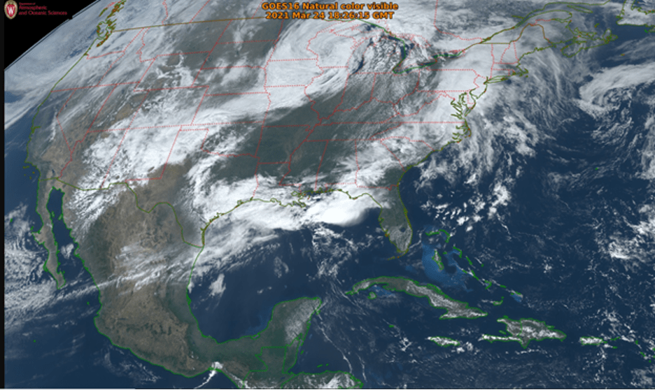
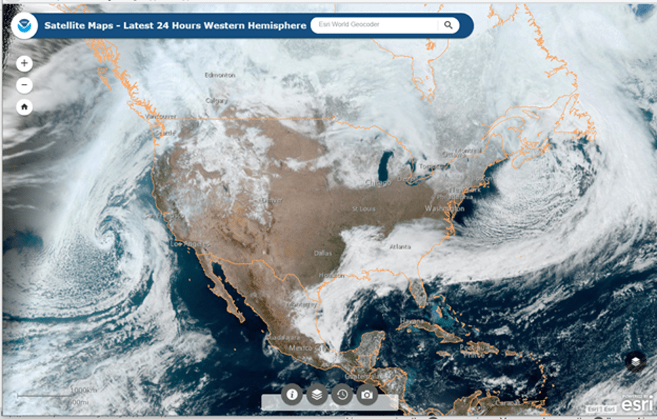
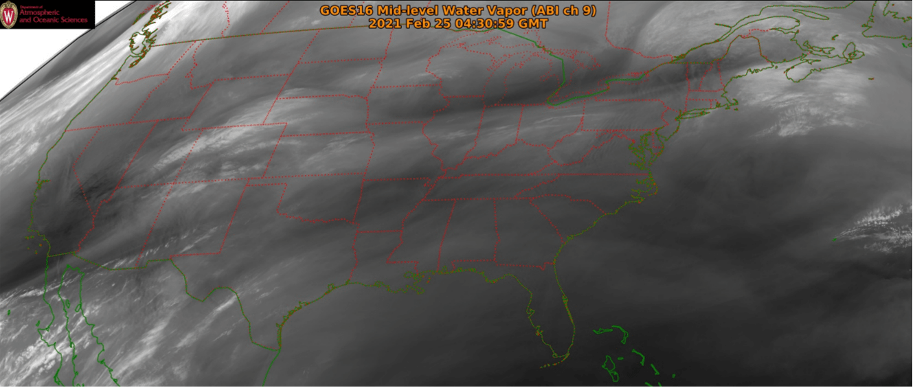
Wednesday March 31st brough another chance for severe weather across much of the Southeastern United States. While this week did not bring a 3rd consecutive SPC issued high risk area, the SPC did issue a slight risk spanning from southern Louisiana and Mississippi to North Carolina (Figure 1). The main reason for this convective activity was due to a cold front propagating eastward. This front was associated with a low-pressure system centered over the Mid-Atlantic. The convection associated with the front can easily be seen in the visible satellite imagery (Figure 2). White clouds associated with convective activity can be seen extending from Louisiana northward along the East coast, into Canada. The visible imagery does not clearly depict a low-pressure system with a classic counterclockwise flow, and the reason for this is due to a surface cyclone in Southeastern Canada with a cold front extending southward into the US. The interaction of convection with this system and the Mid-Atlantic system makes for a messier visible image.

Figure 1: SPC convective Day 1 outlook for the United States. This outlook was for 31 March 2021 13Z to 01 April 2021 13Z. Fill pattern displays outlook type. Image courtesy of the NOAA/NWS Storm Prediction Center.

 

Figure 2: This is a visible satellite image from GOES-16 at 18Z 31 March 2021. Image courtesy of University of Wisconsin-Madison.

 

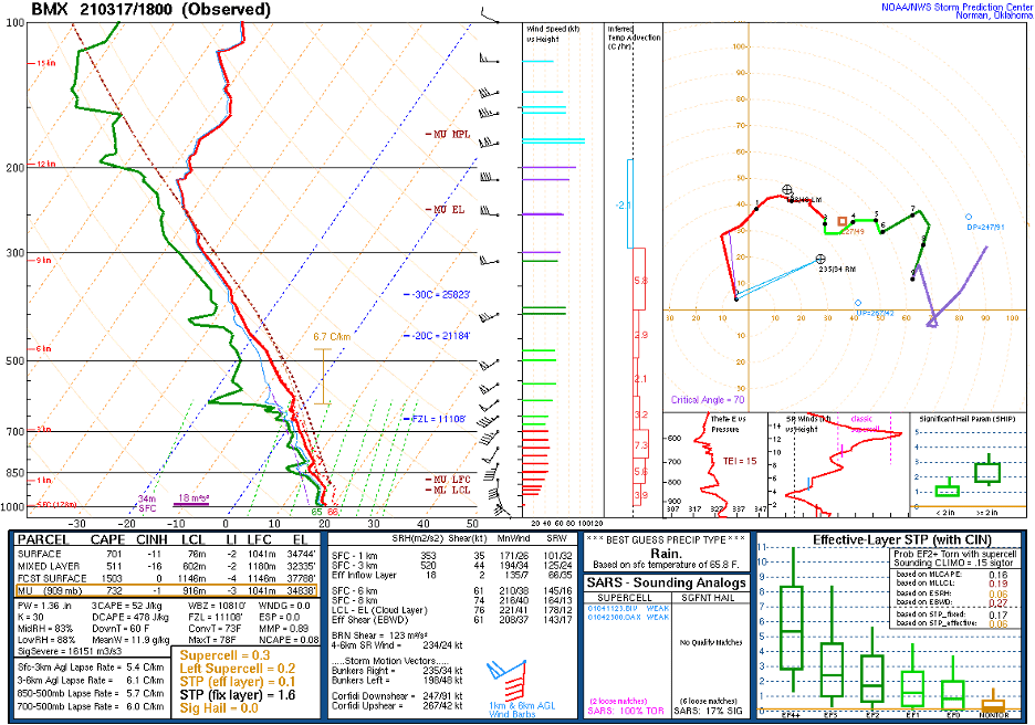
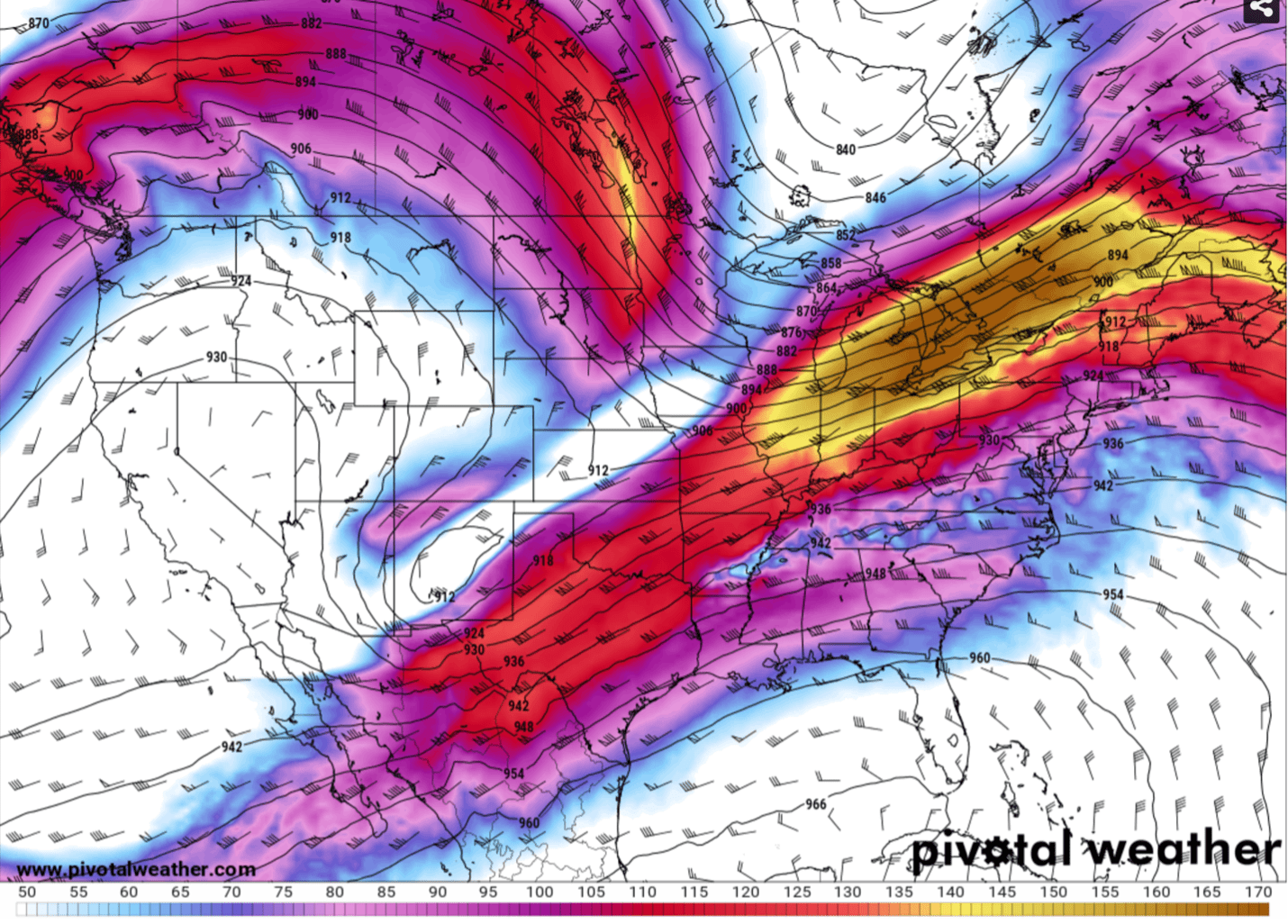
The reason the Southeastern US had a slight risk for severe weather was due to a variety of synoptic and mesoscale factors. Water vapor satellite imagery can provide more insight about the position of the jet stream and associated jet streaks. On water vapor imagery, the jet stream can be identified by looking for contrasting bright and dark regions. Along this border is where the jet stream will be. Additionally, there are four indicators of jet streaks on water vapor imagery: 1) Strongest brightness temperature gradient, 2) Transverse banding, 3) Fastest region on animation, and 4) Intensifying ridging. Based on Figure 3A, transverse banding can be seen of the NE coast of the United States. Additionally, a strong brightness temperature gradient is in this region as well. As a result, a jet streak would be expected over the Great Lakes & NE United States into SE Canada. Looking at data from the SPC Mesoscale Analysis Archive from the same time as the water vapor image (1800 UTC), a jet steak is present in the exact region expected (Figure 3B). Much of the SE United States is in the region downstream of the trough, and this region is where mid-tropospheric upward vertical motions occur due to ageostrophic divergence aloft. Additionally, this region is in the right jet entrance region of the jet streak which is also associated with mid-tropospheric upward vertical motions (UVM). This UVM can be confirmed by the purple contours which indicate UVM on Figure 3B.

 

Figure 3A (left) is a water vapor satellite image from GOES 16 at 18Z 31 March 2021. Figure 3B (right) is a 300 mb height (contours, black, mb), wind speed (fill pattern), and divergence (contours, purple) from 31 March 2021 at 18Z. Images courtesy of the University of Wisconsin-Madison and the SPC Mesoscale Analysis Archive.

 

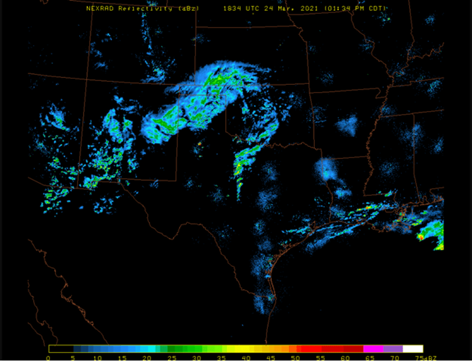
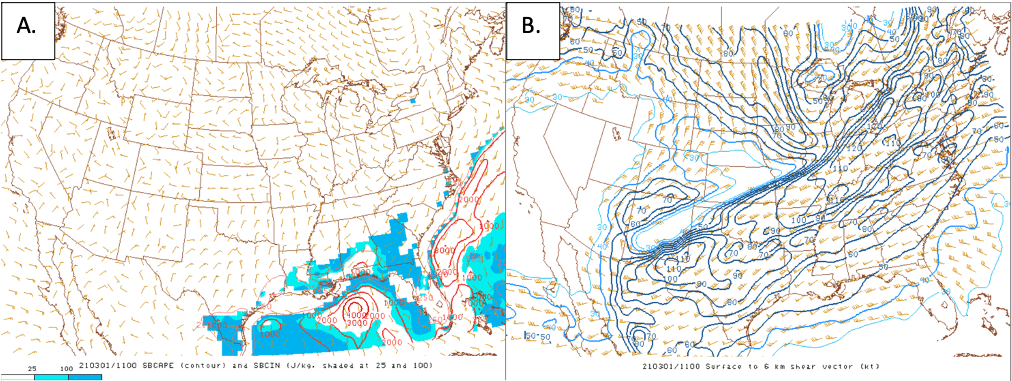
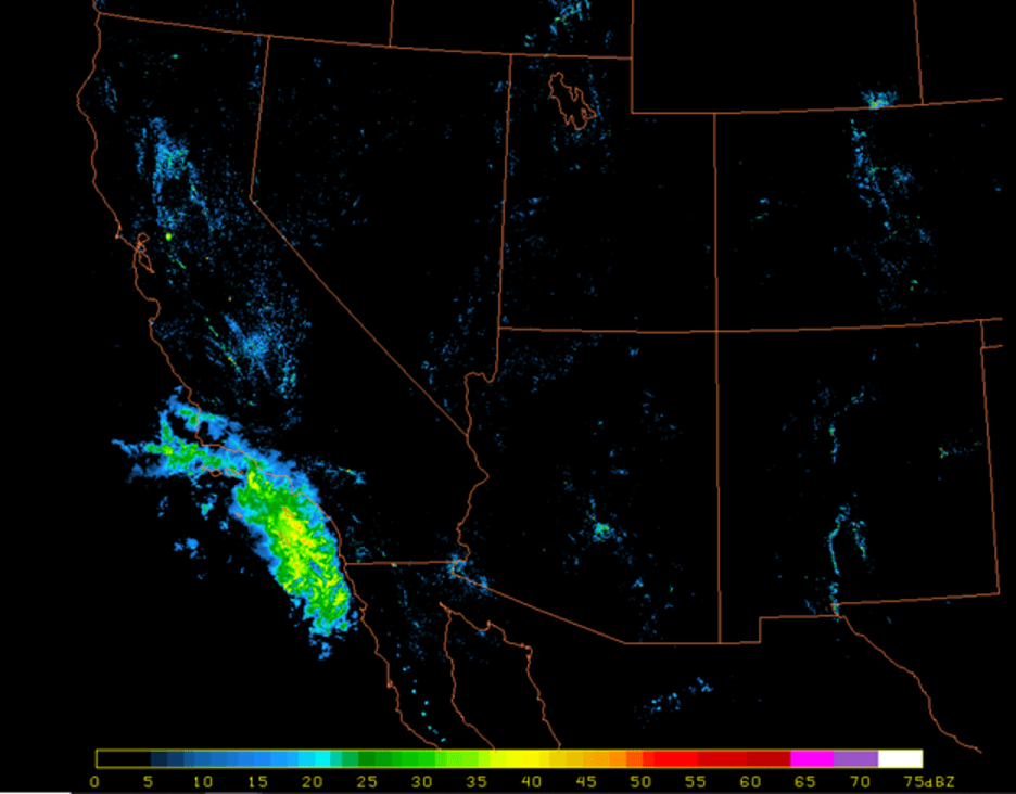
In addition, the mesoscale environment was favorable for convective activity as well. The former water vapor image shows ample moisture over the Southeast, indicated by the white and gray coloring. CIN was present across much of GA and SC around 14Z but dissipated around 18Z. CAPE values ranged anywhere from 250 – 1000 J/kg over the region of interest around 18Z (Figure 4A). In addition, 0-6 km shear values ranged anywhere from 40-60 knots over the region at 18Z (Figure 4B). Supercell composite parameter values were not that impressive at 18Z as the predominant value was .5 (Figure 4C). The moderate CAPE values along with the mild to moderate shear environment were the primary mesoscale factors that led to multicellular thunderstorm development rather than intense severe supercells. This type of convective activity can be confirmed with radar reflectivity data from March 31st. The data shows the most intense convection and precipitation ahead of the front, with lighter precipitation lagging behind (Figure 5).

 

Figure 4A (top left) is a plot of CIN (fill pattern, shaded at 25 and 100 J/kg) and CAPE (contours, red, J/kg) from 31 March 2021 at 18Z. Figure 4B (top right) is a plot of 0 -6 km wind shear (contours, blue, knots, every 10 knots) from 31 March 2021 at 18Z. Figure 4C (bottom) is a plot of Supercell Composite Parameter (contours, blue) from 31 March 2021 at 18Z.

 

Figure 5 is radar reflectivity data from 31 March 2021 at 21Z. The fill pattern (dBz) represents precipitation and its intensity.

 

Overall, the Southeast United States was situated in a mild area of instability in regard to the synoptic and mesoscale environments. The jet streak present over the Northeast was strong but positioned just a bit too far from the SE to maximize UVM in the region. Had the shear environment been more intense, a severe weather outbreak with supercells could have occurred, but the mild shear coupled with moderate mild to moderate CAPE was not enough.

A potent severe weather outbreak with all hazards (including strong tornados) was on tap for the South during the day and night of Thursday, March 25th. IR imagery from the morning showed thunderstorms already underway across portions of MS/AL based on very bright white spots over the area indicating cold cloud tops with discrete cells among the convection. The environment was primed for severe convection starting the night before on the 24th across parts of AK-LA-TX. Figure 1 depicts a supercell thunderstorm that formed near Junction, TX that at the very least developed some rotation based on velocity imagery (bottom panel) that showed a red-green

Figure 1: Radar Reflectivity (top) and Velocity (bottom) from KSJT (San Angelo, TX)

 

couplet just west of the Junction area. Red colors indicate winds moving away from the radar while green colors indicate winds moving towards the radar, and when these two colors show up adjacent to each other and oriented in a tight couplet this indicates rotation. A corresponding hook echo is observed on radar reflectivity (top panel) just southwest of Junction where the possible tornado may have formed. A possible hail core associated with the supercell is indicated by the pink colors (this indicates very high dBZ values associated with large hydrometers such as hail).

The environment producing strong thunderstorms that night and through the day on Thursday the 25th was highlighted by a very warm, moist and unstable airmass over the deep South. In order to see this more clearly, I have included a screenshot of RGB Airmass imagery (Figure 2). This type of imagery is meant to identify all the different kinds of airmasses across a region. Specifically deeper green colors indicate a warm, moist airmass which one can see is draped across the South. A lot of this warm moist

Figure 2: Airmass RGB Imagery from ~21z Thursday, March 25th

 

air is being supplied by a subtropical jet feature that set up over the Gulf of Mexico, bringing a constant stream of moisture into the region, resulting in high 60’s to low 70’s dewpoints across the area (Figure 3). Based on figure 3, a cold front was along the Mississippi River around 21z and looking at RGB Airmass imagery, you can see where some orange colors are found amongst the green around that same area. Orange colors indicate drier air and while not the best indicator of where the cold front is, it does

Figure 3: 21z Surface Analysis from WPC

 

hint a little at where the transition from a moist airmass to a dry airmass could be taking place. As you look to the west of the cold front you can see where dewpoints are starting to lower significantly which also hints at the drier airmass in the wake of the front. Not only do these orange colors on Airmass RGB indicate drier air, but also where a possible jet stream might be as well as any vorticity anomalies that can play a significant role in the overall dynamics of severe convection.

One way to figure out where the jet stream or upper-level trough feature is on RGB imagery is to look for deeper orange colors. Figure 2 not only shows this across the Eastern Plains and into the Midwest, but the shape and curl from the observed orange colors outlines the shape of the upper-level trough feature that was present that day. This trough was responsible for a lot of the upper-level divergence occurring which led to strong upward vertical motions and lift in the lower troposphere which helped to build and maintain the severe convection that day. Another feature to point out with those oranges colors is the present of strong vorticity anomalies. Vorticity anomalies are associated with dry, stratospheric air penetrating the troposphere which is what the orange colors on Airmass RGB imagery represent. Figure 4 is from the Alisha Bentley map analysis site showing relative vorticity values at 500mb as well as geopotential

Figure 4: 00z Friday, March 26th 500mb Relative Vorticity (Alisha Bentley),
heights (black contours), rel. vorticity (fill pattern), ascent (blue)

 

height values at that level. Around the same area as the orange colors in figure 2 is where the trough feature is further outlined by the geopotential height contours. Within this region there are high values of vorticity and because the geostrophic wind can advect higher values of vorticity into a region, if you follow the height contours you can see where this vorticity is moving towards. Values of higher vorticity advecting into regions of lower vorticity is known as positive vorticity advection (PVA). PVA is generally associated with enhanced upward vertical motions and wind shear. Based on figure 4 there are high values of vorticity moving into the Midwest and South and therefore strong upward vertical motions can be expected in these areas as indicated by all of the blue showing up in these regions. This was one of the key ingredients fueling the severe weather outbreak that occurred that day across a large section of the country. This combined with the very warm, moist and unstable airmass led to an eruption of severe weather in the Midwest and especially across the South.

On Wednesday, March 24th, 2021, a low-pressure system moved across the Southwestern United States dropping much needed precipitation in the forms of both rain and snow in the area. As seen in the visible satellite image in Figure 1, the low-pressure system targeted New Mexico and the Four Corners region of the United States. In this image, you can see that the low-pressure system in question does not exactly have the defined comma shape of a typical extra-tropical cyclone, especially in comparison to the stronger low-pressure system that curls up the east coast and up around the Great Lakes region. The reason for the lack of this typical shape could be due to a couple different reasons including the weak nature of this system or the current location of the system being far from an oceanic source of moisture. Although it was not the strongest system, the precipitation it brought was incredibly important due to the severe drought that this region is experiencing, especially moving into the warmer seasons of spring and summer.

Figure 1: Visible Satellite Imagery (UW Madison) at 18Z on March 24th, 2021 showing the low- pressure system sitting over New Mexico and the Four Corners region.

 

To further analyze the strength and moisture associated with the system, we can look to the water vapor satellite imagery shown in Figure 2. Looking at the Southwestern U.S., you can clearly see the bright white and light gray signatures associated with high to moderate moisture content in the clouds. These colors clearly show the presence of a system that is expected to bring some precipitation to the area. Another notable feature on this image, is the dry streak that dips southward and then curves northward around the low. The clear color gradient between the dry, black air and the moist, light air reveals that this is the location of the jet stream, and more specifically a trough supporting this surface low. It is also interesting to note the large dark streak cutting through the southeast in between the two low-pressure systems, creating a moist, dry, moist pattern across the continental United States.

Figure 2: Water Vapor Satellite Imagery (UW Madison) 18Z March 24th, 2021 showing the moisture levels associated with the low over the Southwestern United States.

 

To decipher the intensity and type of precipitation expected from this system, we can look at the radar image shown in Figure 3. In this image, you can see a clear patch of blue and green reflectivity centered over New Mexico and Texas. Cooler colors, such as green and blue, are associated with less intense precipitation than the warmer colors, such as yellow and orange, indicating that this low-pressure system is associated with lower intensity precipitation. To help determine which type of precipitation is falling, you can look at whether the signature appears smoother in nature or rougher/defined. As seen around the northern edge of the storm, the smoothness indicates that the precipitation dropped in this area is in the form of snow. However, more towards the south of the storm, there are pockets of yellow more defined signatures that represent higher intensity rain precipitation. However, not every signature on a radar reflectivity map indicates precipitation. The sporadic blue spots you notice on the image are called false echoes and are a result of reflection off of a building, landform, or other large object.

Figure 3: NEXRAD Radar Reflectivity Image (UW Madison) at 18Z on March 24th, 2021 showing reflectivity values for the system over the southwest.

 

Finally, we can look at Figure 4 to dive into the human impacts of this extra-tropical cyclone, both positive and negative. The image on the left shows the current hazard warnings issued by the National Weather Surface around 18Z on March 24th while the image on the right shows the individual reports of precipitation, winds, and property damage. There is a clear conglomeration of both warnings and reports centered over New Mexico where the low-pressure system dropped most of its precipitation. On the left, the purple regions represent winter weather advisories while the pink regions represent winter storm warnings. It is also interesting to note the thin region with no warnings through the center of the state which was most likely unaffected due to lower altitudes. On the right, the gray symbols represent observed snow, the green represent observed rain, and the blue and red representing high winds and wind damage respectively. These reports correlate well with the data we observed on radar of both snow and rain precipitation in the region. Across the state, the snow ranged from 0.2 inches to 6.5 inches at 18Z, and the wind gusts ranged from 55-65 miles per hour proving that even a weaker low-pressure system can bring serious impacts.

Figure 4: Current Hazards and Observation Reports (National Weather Service) at 18Z March 24th, 2021.

 

Even though it appeared late in the winter storm season, this low-pressure system was impactful to the Southwestern United States as it brought much needed precipitation to the dry Four Corners region. The final totals of snowfall in New Mexico ranged from 6 to 16 inches in some of the higher altitudes, providing some drought relief for the region as the dry summer months approach. After moving through the southwest, this low dissipated and moved eastward across the United States continuing to drop minimal precipitation in the form of rainfall.

A squall line brought severe thunderstorms and tornadoes to Alabama and Mississippi Wednesday night and early this morning. Storms will continue to move east through Georgia, the Carolinas, and parts of West Virginia later today, producing more severe weather later this evening. The Storm Prediction Center’s Day 1 Convective Outlook (Figure 1) shows the current tornado risk for today associated with this storm system.

Figure 1: SPC Day 1 Convective Outlook

 

Tornado watches are currently in effect across southern Georgia and the Florida panhandle as a well-defined squall line moves through the area, as spotted on radar shown by Figure 2. This squall line formed along the cold frontal boundary of an extratropical cyclone (as seen in Figure 3) developing across the US. The red colors on radar correlate to the most severe aspects of the storm such as tornadoes. Radar can be used to identify the debris ball of a tornado and the classic hook shape of a supercell. Supercells usually develop ahead of a cold front, so now that the squall line has formed, less supercells are moving through Georgia.

Figure 2: NEXRAD Radar Reflectivity

 

Figure 3: GeoColor Satellite Imagery, currently showing multispectral infrared imagery

 

However, this storm system is well supported by an upper-level trough and strong jet stream as shown in Figure 4. As this trough moves east across the US, winds are expected to pick up, increasing shear, giving these storms the potential to develop back into supercells in the Carolinas. After the trough moves through continental US, a zonal flow pattern appears regionally in the Southeast, bringing clear weather and the conclusion of this area’s severe weather.

Figure 4: 250mb Wind Speed

 

Infrared satellite imagery in Figure 5 shows bright green clouds along the squall line and over Indiana, Illinois, Ohio, Michigan, and Kentucky. These green colors correlate to the coldest temperatures of clouds, indicating where the thickest clouds are and relating to areas of strong convection. Indiana, Illinois, Ohio, and Kentucky are expected to receive thunderstorms as the warm front of the northern side of this extra-tropical cyclone develops throughout the day and moves through the area.

Figure 5: Infrared Imagery

 

Sources:

Figure 1 https://www.spc.noaa.gov/products/outlook/day1otlk.html

Figure 2 https://tempest.aos.wisc.edu/radar/se3comphtml5.html

Figure 3 https://www.star.nesdis.noaa.gov/GOES/conus_band.php?sat=G16&band=GEOCOLOR&length=48

Figure 4 https://www.tropicaltidbits.com/analysis/models/?model=gfs&region=us&pkg=uv250&runtime=2021031712&fh=0

Figure 5 https://www.star.nesdis.noaa.gov/GOES/conus_band.php?sat=G16&band=11&length=60

On March 15th the National Weather Service put out a convective outlook for the next day with a prediction for a slight risk of convective activity over Kansas, Oklahoma, and a part of Texas and marginal risk and risk of thunderstorms as far North as Iowa and as far East as the Carolinas. Those risks manifested in wind, hail reports, and tornadoes. The system that was the source of these intense thunderstorms was an extratropical cyclone that was supported by a low-level jet stream. Focusing on the 925 and 850 millibar levels at 12Z on March 16th, there was a clear trough feature that was situated over Texas and several other Great Plane states. The trough feature can be directly correlated to this initial round of intense thunderstorms and supercells, due to the fact that rising motion forces air into the tropopause can lead to strong updrafts and thus strong thunderstorms near the troughs. This can lead to increased convective activity and an increased chance of intense precipitation and convective activity.

 

On the 16th of March, another convective outlook was produced by the Storm Prediction Center with not only enhanced and moderate risks for severe thunderstorms but also an area of high risk over Alabama, Mississippi, and parts of Louisiana and Missouri. The reason that a high convective outlook is so significant is because they are so seldom issued. As a matter of fact, the high convective outlook issued on the 16th of March, was the first one issued since 2020. By the 17th, the trough feature had deepened and the low-level jet at both the 850 and 925 millibar levels had strengthened. This allowed for not only shear, with the increasing wind speed and change in direction with height, but also allowed for the acceleration of the movement of any supercells that formed. Additionally, when examining the Skew-Ts many of the aspects of instability that are necessary for severe thunderstorms were present in the atmosphere: shear, CAPE, lift, and thermodynamic instability. Some of these elements are not evident in the Birmingham sounding at 18Z, but the some of the other elements on the sounding, such as the Bulk Richardson Number for shear was 123 m^2/s^2, a value indicative of high potential for supercell thunderstorms and intense thunderstorms.

Birmingham, Alabama sounding at 18Z on March 17th, 2021

 

On the 16th of March, according to the Storm Prediction Center, there were three tornado reports, the strongest one reported being EF1, 48 wind repots, and 55 hail reports. On the next day, there was a great amount of suspense waiting for the first warnings and watches the first being issued at 1243 UTC in Northwestern Mississippi. The 17th of March had 56 tornado reports, the strongest being an EF2, a total of five injuries, 102 wind reports, and 49 hail reports. This was a destructive storm system that has the potential to cause damage and did. The subsequent days of this extratropical cyclone also brought damage and destruction to areas on the East Coast.

By Thursday morning, the low pressures system, which was centered over the northern part of Wisconsin, has moved northwest and is now centered over Lake Superior and southern Ontario. As seen in the surface analysis map below, this system is producing an associated cold front, which is producing storms over the Midwestern states, producing the strongest storms over the states of Illinois and Indiana. The system has a minimum pressure of around 993 mb, which is about the same pressure the system had the night before. The pressure gradient around the surface low appears to have strengthened as the isobars have moved closer together. Figure 2 shows a black and white visible satellite image of the system.

Figure 1: Surface Analysis Map 11 Mar 1200Z

 

Figure 2: GOES-East Visible Satellite Image, 11 March 2021 13Z

 

Figure 3 shows the GOES-East Infrared Image of the system. This image is overlayed with associated radiative temperature of the system. When viewing infrared images, the whitest regions are associated with the coldest radiative temperatures. This also gives us insight into the cloud height and convective energy of this system. The whitest (coldest) regions on the map indicate clouds that have pushed further up into the atmosphere, which is usually associated with higher convective activity. In the figure below, you can see somewhat cold temperatures associated with the system over the Midwest. This indicates that clouds in this region have pushed higher into the atmosphere, and there is some convective activity associated with this system.

Figure 3: GOES-East Infrared Image, 11 March 2021 13Z

 

Figure 4 shows the radar image of this system at 13Z. The radar shows a loosely-organized group of storms over the Midwest to eastern US. The strongest storms of this system are centered over Illinois and Indiana, where a squall line can be seen running from St. Louis to just west of Indianapolis. The squall line runs parallel and just out in front of the associated cold front seen on surface analysis map in Figure 1. Overall, the low-pressure system, and its associated cold front, is producing storms with moderate precipitation and intensity.

Figure 4: Radar, 11 March 2021 13Z

 

Based on the position of the low-pressure system, I believe it will continue to strengthen throughout the day today. It is located between a downstream trough and an upstream ridge. This is an area of divergence and upward vertical motion, which is conductive to the strengthening of extratropical anticyclones, such as this system. On Figure 4 below, the system can also be observed to be in the left exit region of the jet stream, which could also be a source of strengthening for this system. I believe this system will continue to strengthen and produce more organized storms as it moves east to northeast throughout the day.

Figure 5: 300 mb Observation Map, 11 March 2021 12Z

A low-pressure system brought significant rain to Southern California on March 10th and March 11th. At the time of this presentation, the system was right at the peak of its strength and beginning to degenerate. Part of the reason for this was the placement of the subtropical jet stream as seen below in figure 1, the mid-level water vapor satellite image. The jet looked to be positioned just south of California going into Arizona. It is possible to spot because though not shown in the image, the clouds in the area where the jet was were moving faster than the other clouds in the region. Additionally, a slight ridge was beginning to form on top of transverse bands, which are ripple-looking clouds close to the jet. You can see them if you look across middle west Texas. A map of upper-level wind patterns confirms this in the second panel of figure 1.

Fig. 1: (top panel) A mid-level water vapor satellite image (source: https://whirlwind.aos.wisc.edu/~wxp/goes16/wv/goes16_namer.html)  from 11 March 2021 at 12:10 UTC, and (lower panel) is a wind mat at 250 mb with sea level pressure contours in black, 1000-500 mb thickness in red and blue dashed lines, and the wind speed shaded based on the color bar (source: http://www.atmos.albany.edu/student/abentley/realtime/standard.php?domain=northamer&variable=mslp_jet)

 

California is currently in a drought, and they are almost to the end of a drier than average wet season. Due to the drought gripping the state, any precipitation is welcomed at this point. This was a good soaking rain over the course of multiple days. There were a few mudslides reported nonetheless. Snow was even recorded at higher elevations in the mountains. Both Los Angeles and San Diego recorded over half an inch of rain, and San Diego was 0.43 inches above average for the rainfall expected for the March 11th. Below in figure 2 is the forecasted amount of rain for the areas.

Fig. 2: This is a map of 24-hour Qualitative Precipitation Forecast totals. It was issued March 10th at 08:32 UTC and forecasted for 12:00 UTC March 10th to 12 UTC March 11th. The color scale indicated California could receive anywhere from 0 to 1.25 inches of rain depending on the region. (source: https://www.wpc.ncep.noaa.gov/archives/qpf/display_maps.php?prodtype=issued&proddate=03/10/2021&prodtime=12&allsent=no&imagetype=color&actualprods=94q)

 

This system had output most of its precipitation by March 11th, but some precipitation remained. The progression of the system over radar was fascinating to watch because it did not look too impressive. The key to remember is if it were a system over the Midwestern plains or the east coast, the system would not mean much. Because it is California, people had to be reminded to drive more carefully than they were used to and prepare for a rain shower like the southeast U.S. prepares for a snow shower, minus purchasing the milk and bread. Here is a clip of a meteorologist giving the weather report on March 10 just before 17:40 PST (01:40 UTC) (source: https://www.foxla.com/video/909367)

https://www.foxla.com/video/909367

 

 

While it was a relatively quiet weather week across most of the United States, a squall line that moved through Georgia during the early hours of Monday, March 1st spun up a quick EF-1 tornado in Clayton County around 1100 UTC. The tornado only lasted about ¾ of a mile and was on the ground for less than a minute. The WPC surface analysis map from 09Z March 1st, 2021 shows a cyclone centered over Eastern Canada (Figure 1). A cold front extends from the center of this low to the southwest where it ends in Texas. This front will serve as the lifting mechanism for storms to develop as it marches through the Southeast.

Figure 1: WPC surface analysis map of the United States from 09Z 1 March 2021. Source: WPC Surface Analysis Archive

 

The synoptic scale environment, or large-scale atmospheric environment, was favorable for cyclone maintenance and strengthening at this time. The reason for this is because of two main features at play: a trough located over the Great Lakes Region and a jet streak over the Northeastern US and into Canada (Figure 2). The surface cyclone was located downstream of the trough, an area where air diverges, or spreads outward, aloft. This causes air from the mid-troposphere to fill in the gap where the previous air above was, inducing upward vertical motions. This in turn strengthens the low-pressure system. In addition to this, the cyclone is located in a favorable environment for strengthening with respect to the jet streak. The cyclone is located in the left jet exit region, which is also a region where air diverges. For the same reasons as the trough, this will induce upward vertical motions and enhance the surface cyclone.

Figure 2: Model displaying 300 mb height (black contours, dam) and wind speed (fill pattern, knots) from 09Z 1 March 2021. Source: Pivotal Weather

 

While the synoptic environment is favorable for surface cyclone strengthening, this cannot be attributed to the development of the tornado because the surface cyclone is so far away from GA. The mesoscale environment, or smaller-scale atmospheric conditions, must be analyzed to see what led to this short-lived EF-1 tornado. Two key variables in the mesoscale environment can be looked at to determine how unstable the atmosphere was around the time the tornado formed. The first variable is convective available potential energy (CAPE). CAPE is essentially how much “fuel” there is in the atmosphere for the thunderstorm to use. At 11Z, no significant values of CAPE were present over Clayton County (Figure 3A). Since CAPE was not a factor, something else must have led to an unstable environment to allow for this tornado. The second variable that will be analyzed is 6 km wind shear. Shear values of 60 and 80 knots are seen across Central and North Georgia at 11Z (Figure 3B). Even with little to no CAPE, this strong shear environment is sufficient enough for a tornado to form.

Figure 3: This panel displays mesoscale variables used in determining atmospheric instability. Figure 3A displays SBCAPE (red contour, J/Kg, 1000 J/kg intervals) and SBCIN (fill pattern, shaded at 25 and 100 J/kg) at 11Z 1 March 2021. Figure 3B displays 6km wind shear (blue contours, knots, 10 knot intervals) at 11Z 1 March 2021. Source: SPC Mesoscale Analysis Archive

 

Now that we understand the role the synoptic and mesoscale environments played in forming this tornado, satellite and radar imagery can provide us a clear image of exactly what happened and where it happened. Composite radar reflectivity imagery allows us to track the precipitation within the squall line and see how intense it is (Figure 4). The squall line feature is clearly identified in this imagery as the band of red and yellow. These colors are associated with higher dBZ values (larger rain droplets) which indicate more intense precipitation. This radar image shows the squall line moving to the southeast with lighter precipitation trailing behind. Not only can radar provide information about precipitation, but radial velocity imagery can provide valuable information on the motion of air in the atmosphere. The radial velocity image depicts primarily blue and red coloring where blue indicates motion towards the radar and red indicates motion away from the radar (Figure 5A). The motion of the system appears to be northwesterly based upon the shading pattern, and this can be confirmed by surface wind data (Figure 5B). In addition, radial velocity imagery can be very useful when identifying tornadoes in a supercell because the rotating air will appear as a tight region of blue and red on the image. While the tornado event on Monday was not from a supercell, the radial velocity imagery still displays a region of instability around Atlanta as indicated by the region of blue and red shading. This region of instability is near Clayton County where the tornado on Monday occurred. By looking at the synoptic and mesoscale environments along with radar imagery of the actual event, it can be better understood why an EF-1 tornado spun up in Clayton County GA.

Figure 4: This is a loop of composite radar reflectivity data (fill pattern) from 9:55Z to 11:55Z on 1 March 2021. Source: UCAR Image Archive

 

Figure 5: This panel displays radar data along with modeled surface wind data. Figure 5A displays radial velocity data (fill pattern). Figure 5B displays surface wind magnitude and direction (wind barbs) and surface temperature (fill pattern). Source: NCAR and Pivotal Weather

On Wednesday, March 3rd, 2021, a low-pressure system was making its way towards the West Coast, targeting Southern California and Northern Mexico. The low-pressure system was not very strong as it approached the coast with a pressure of 1006 mb and was only expected to drop between 0.01 inches and 0.10 inches of precipitation. However, any precipitation is welcome in this area of the country as it is typically very drought ridden. This system was very well defined as you can see in the visible satellite imagery in Figure 1 with a clear frontal boundary curling into a hook at the top of the system. Visible satellite imagery shows what one would see with their eyes from space, so the colors and features on the map are true to their actual appearance on Earth.

Figure 1: Visible Satellite Imagery (NOAA) 15z March 3rd, 2021

 

To further explore the strength of the system, we can look to the infrared satellite image shown in Figure 2. On an infrared satellite image, the clouds that are higher in the atmosphere and therefore colder appear brighter white, while the clouds that are closer to the ground and warmer appear darker gray. As you can see in Figure 2, there is not a great contrast of color between the low-pressure system we are analyzing and the ocean, meaning the clouds are lower to the ground and warmer than we would usually expect out of a low-pressure system. Since the clouds do not reach as far up into the atmosphere, that indicates that there is little to no convective activity that would produce events such as severe thunderstorms.

Figure 2. Infrared Satellite Imagery (UW Madison) 15Z March 3rd, 2021

 

Since the biggest impact of this low-pressure system to the human population was the precipitation aspect, we can turn to the radar reflectivity image as shown in Figure 3 to help decipher the intensity and type of precipitation that was expected from this storm. Although the radar does not specifically distinguish rain from snow, there are a few ways you can better tell them apart. Areas with cooler colors and a smoother appearance indicate a snow or mixed precipitation event while warmer colors and a more defined appearance indicate rainfall. In Figure 3, which displays the low-pressure system hitting the California coast, you can see there are some areas of more intense rainfall indicated by the yellow and small pockets of orange. However, if you look to the Northern portion of the system, the signature appears blue and smoother in nature indicating that the precipitation was falling as snow in the mountains of Southern California. Another feature on radar to note is all the dispersed blue areas shown sporadically across other states. These could easily be mistaken for signatures of precipitation; however, they are most likely false echoes being returned to the radar from buildings, landforms, or even large groups of insects or birds.

Figure 3. NEXRAD Radar Reflectivity Imagery 18Z March 3rd, 2021

 

The strength of a low-pressure system can also be analyzed by going up much higher in the atmosphere, around 250 mb, and looking at how it is supported by upper atmosphere winds and the jet stream. As shown in Figure 4, the jet stream is indicated by the colors with blue being slower wind speeds and the darker pink being faster wind speeds. The pockets of the darker pink color are known as jet streaks which are known for their very fast winds and supporting stronger systems. Looking off the coast of California, it is clear that the low-pressure system is supported by a trough and upper-level winds, but not by any major jet streak. This matches up with the conclusion we came to previously that this low-pressure system was of a weaker nature. Another interesting phenomenon to note on this map is the split flow of the jet stream across the continental United States. There are two major jets that interact across the United States, the polar jet and the subtropical jet, and you can clearly see the two split off from each other and then join back together off the East Coast.

Figure 4. 250 hPa Jet Stream (Alicia Bentley) 12z March 3rd, 2021

 

Ultimately this low-pressure system, while well-defined in shape, was overall a fairly weak system. However, it was impactful in the sense that it brought much-needed precipitation to Southern California, about 1/10th of an inch to be exact. Once the system dropped its precipitation, it quickly dissipated and broke apart as it moved inland over the Rocky Mountains, limiting the impact it would have on the rest of the country.

A low-pressure system over the Great Lakes brought a cold front across the Northeast US along with some rain and snow. At 12Z 24 February, this low-pressure system was perfectly positioned in the right jet entrance region of the jet streak, indicated by the dark pink color, shown in Figure 1.

Figure 1. 250 mb map, best used to identify upper-level wind, specifically the jet stream

 

Low pressure systems are characterized by air converging, or coming together, at the ground and then rising. The right entrance region of a jet streak is characterized by divergence, or air moving apart, at high altitudes. When stacked above each other, these conditions are optimal for the low be maintained as it moves away from the Great Lakes and across the Northeast US. Figure 2 shows how divergence and convergence are related to high- and low-pressure systems.

Figure 2. Diagram of air flow in high- and low-pressure systems

 

Figure 3 is a surface analysis showing the low and its associated cold front at 18Z 24 February. Cold fronts and low-pressure systems appear hand in hand because the cold, denser air lifts warmer, less-dense air. This rising air creates an area of low pressure that is often associated with rain and thunderstorms. Rain was present along the cold frontal boundary, but this specific front was weak enough that no severe weather impacted the area. However, snow did occur along the warm frontal boundary east of the low. While this seems like a juxtaposition, warm fronts do often produce snow in winter due to their less aggressive nature than cold fronts.

Figure 3. NAM surface analysis map

 

As the front continues to move across the Northeast, it continues to stay fairly weak. The temperature gradient as seen on the surface observations in Figure 3 is not super strong. This is supported by the water vapor satellite imagery show in Figure 4 and the air mass RGB in Figure 5. When looking at water vapor satellite imagery, darker colors indicate lack of moisture in the atmosphere while lighter whites represent more moisture. As you can see in Figure 4, this front is also not associated with strong moisture gradient; higher contrasts have been seen throughout history.

Figure 4. GOES 16 water vapor satellite imagery

 

Drier, colder air will follow behind the frontal boundary, but it will not be highly different than the warmer, moister air in front of it as seen in Figure 5. In air mass RGB imagery, green colors represent warmer, moister air with blues and purples indicating cooler, drier air. The air following the cold frontal boundary is only slightly bluer than the green air before it. The cold front is expected to continue moving across the Northeast and into the Atlantic Ocean over the next couple days, bringing cooler temperatures to the region.

Figure 5. GOES 16 air mass RGB

 

Finally, I would like to note that the lack of severe weather across the rest of the United States is due to the impressive zonal flow spanning the height of continental US and the positively tilted trough over the western US as seen in Figure 6. Positively tilted troughs produce little severe weather, and zonal flow is associated with moving storms associated with cold fronts fast across the US just like this cold front in the Northeast.

Figure 6. 250 mb wind imagery from 2Z 25 February

 

Sources:

Figure 1: http://www.atmos.albany.edu/student/abentley/realtime/standard.php?domain=conus&variable=mslp_jet

Figure 2: https://weatherworksinc.com/news/high-low-pressure

Figure 3: https://www.wpc.ncep.noaa.gov/html/sfc-zoom.php

Figure 4: https://whirlwind.aos.wisc.edu/~wxp/goes16/wv/goes16_conus.html

Figure 5: https://whirlwind.aos.wisc.edu/~wxp/goes16/multi_air_mass_rgb/goes16_conus.html

Figure 6: https://earth.nullschool.net/#current/wind/isobaric/250hPa/orthographic=-87.24,40.51,705