

Hello, I’m Prof. Charlie Kemp. This website has open course materials for Introduction to Biomechanics, a class I’ve taught at Georgia Tech in the Department of Biomedical Engineering since the spring of 2008. On this website, you can access materials from the spring term of 2017 and the fall term of 2022.
BMED 3400: Intro to Biomechanics (Spring 2017)
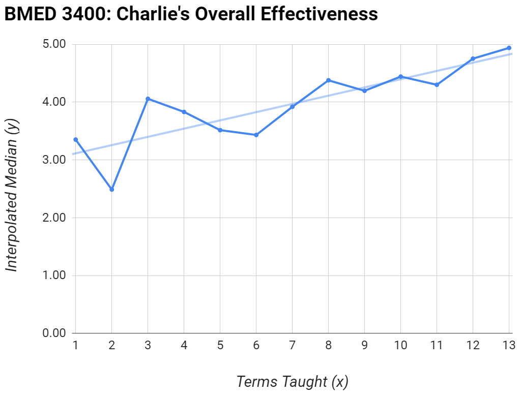
I taught an older version of the course, BMED 3400, for thirteen terms from the spring of 2008 to the spring of 2017. It was a long iterative learning process for me as an instructor (see chart). I then took a leave of absence to co-found a company.
You can download materials from the Spring of 2017 using the links below.
- problems with solutions
- lecture notes
- equation sheet
- reference charts for models of axial loading, torsional loading, and bending
- links to online interactive calculations using Desmos
- links to editable Overleaf documents
- short presentation on teaching that I gave to BME faculty
BMED 3410: Intro to Biomechanics (Fall 2022)
Now, I’m helping teach a new version of the course, BMED 3410, with Prof. Denis Tsygankov and Prof. Scott Hollister. I’ve been documenting the class below. You can also download slides, problems and other materials from the following directory.
Directory with Open Materials from BMED 3410 – Fall 2022
Table of Contents
- Problem-Solving Studio 1: The Meta-Problem-Solving Studio
- Lecture 1: Course Overview and Statics 1
- Lecture 2: Statics 2
- Problem-Solving Studio 2: Statics
- Lecture 3: Model of Simple Axial Loading 1
- Lecture 4: Model of Simple Axial Loading 2
- Lecture 5: Model of Axial Loading 1
- Lecture 6: Model of Axial Loading 2
- Problem-Solving Studio 3: Axial Loading Model
- Lecture 7: Model of Axial Loading 3
- Lecture 8: Statically Indeterminate Systems 1
- Problem-Solving Studio 4: Axial Loading Model
- Lecture 9: Statically Indeterminate Systems 2
- Lecture 10: Review for Exam #1
- Problem-Solving Studio 5: Statically Indeterminate Systems
- The End!
8/22/2022 : The Meta-Problem-Solving Studio (PSS 1)
Since we haven’t had a lecture yet, the graduate student TA (GTA) and I ran a meta-problem-solving studio (meta-PSS). The goal was to design good problem-solving studios based on the students’ prior experiences. Most of the students are in their third year of biomedical engineering (BME) at Georgia Tech, so they’ve had a variety of problem-solving studio (PSS) experiences.
The Department of Biomedical Engineering at Georgia Tech and Emory schedules a weekly problem-solving studio (PSS) for most of its core undergraduate courses. Prof. Joe Le Doux developed the original problem-solving studio starting in 2008 while teaching “Conservation Principles of Biomedical Engineering” (BMED 2210) [1]. You can read about the original PSS and the thinking behind it in the following paper.
[1] Le Doux, J. M., & Waller, A. A. (2016). The problem-solving studio: An apprenticeship environment for aspiring engineers. Advances in Engineering Education, 5(3), 1–27.
While generally true to the original intent, instructors run problem-solving studios with variations. The meta-PSS that the GTA and I ran was valuable because we learned about the students’ preferences from the variations they’ve experienced. The following outline describes what we did during our meta-PSS.
Meta-PSS Outline
- The graduate student teaching assistant (GTA) introduced themself.
- I introduced myself.
- We defined the problem of designing a successful problem-solving studio (PSS) based on the students’ prior experience with PSS.
- We asked students to think about the best PSS experiences they’ve had and use those to provide suggestions.
- I solicited suggestions and led discussions about them.
- The GTA recorded suggestions on the whiteboard.
- Once there were no more suggestions, I used the list of suggestions as design specifications and began designing a prototypical PSS.
- I interactively wrote a PSS schedule on the whiteboard, while soliciting feedback and further discussion, which resulted in further suggestions.
- Once we had an initial design, I asked if everyone agreed with trying it out in for our second problem-solving studio with the understanding that we can iterate our PSS design throughout the term.
- I then set my alarm for a10-minute break during which they talked with one another and the GTA and I talked about the class.
- I then led the PSS through the syllabus using my laptop and the room’s projector while providing my personal perspectives on the content.
Problem-Solving Studio Design Criteria
The design specifications resulting from student experiences were similar to the following. I’ve used boldface for specifications that the students strongly endorsed.
- It should provide opportunities for students to practice communicating the material with one another.
- The problems should be clearly connected to real-world applications.
- Teams should have time to work alone on the problem after it is introduced.
- The GTA and instructor should go over the solution at the end of a problem.
- The GTA and instructor should be available to help teams and individuals.
- The PSS should start with an overview of the material at the beginning.
- Students should have been provided guidance on what to know prior to the PSS.
- A summary of key points should be provided at the end of the PSS.
- Whether or not the PSS is open or closed note should be made clear. Students prefer open note.
- Make sure the problems involve the application of the content being learned.
- Inform students about the expected difficulty of problems.
- Make sure that students have familiarity with simpler problems before moving to more difficult problems.
Out of all the suggestions students made, they were most emphatic about the instructors going over a solution with the entire class at the end of a problem. They expressed that they would prioritize this over other activities, such as students presenting their solutions to the class. Based on the discussion, my impression was that students were sometimes frustrated and ended up leaving a PSS more confused than enlightened. It makes sense to me that they would be primed to learn from a solution presented by an expert just after working on a problem themselves. Presenting a full solution will not always be feasible, in which case the students recommended highlighting key points and approaches to challenges the students encountered.
Initial Problem-Solving Studio Design
The meta-PSS resulted in a problem-solving studio design similar to the following.
- 5 min : Overview of PSS goals with reminder about the content.
- 45 min : Problem #1
- 5 min : Introduce the problem and give guidance on the difficulty.
- 30 min : Each team works alone on the problem while the GTA and instructor cycle around the room.
- 10 min : The GTA and instructor interactively go through the solution while soliciting ideas and questions from the teams.
- 10 min : Class Break
- 45 min : Problem #2
- 5 min : Introduce the problem and give guidance on the difficulty.
- 30 min : Each team works alone on the problem while the GTA and instructor cycle around the room.
- 10 min : The GTA and instructor interactively go through the solution while soliciting ideas and questions from the teams.
- 5 min : The instructor and GTA review of the key points from the PSS.
Each PSS session has 1 hour and 50 minutes available in total. The design above does not provide a safety margin, so the class break and the key points review may be shorter in practice.
Team Formation
In addition, the class discussed how teams would be formed and achieved consensus around the following points.
- Teams are initially based on where people sit. Each table has a team. As such, PSS members become part of a team by sitting at a table.
- Under some circumstances this approach may not result in teams conducive to learning. Forced team mixing can be required by the GTA and instructor under some circumstances, including the following.
- The GTA and instructor believe one or more teams is not functioning well for learning and is unlikely to be significantly improved.
- Team members privately express to the GTA or instructor that they are in a team that is not functioning well for learning and is unlikely to be significantly improved.
- Ideally, mixing the teams will not occur close to an exam. It should ideally occur one or two weeks before an exam.
- PSS members are encouraged to sit in new places if they want to change teams.
8/24/2022 : Lecture 1 – Course Overview and Statics 1
I’ll be giving the first 6 weeks of lectures in BMED 3410. For my first lecture, I started with slides that cover the main goals of the course and then started solving a problem on the whiteboard. In the end, my ideal would be for students to achieve the following course goal.
Course Goal: Learn to Solve Real Biomedical Engineering Problems with Simple Mechanical Models
You can download my slides in various formats via the following links: Google Slides, PDF slides, ODP slides, and PPTX slides.
I began working through a design problem with the class that uses a rigid body model in static equilibrium. The whimsical goal is to design a wearable robot that would enable me to create a YouTube video in which I perform an iron cross on the rings, which is a challenging skill from gymnastics that is well beyond my abilities. This problem was inspired by wearable robotics efforts that seek to augment human performance. Importantly, wearable robotics efforts have also sought to benefit people with injuries and disabilities through rehabilitation and assistance.
We did not finish the problem, but by the end of the class we understood the problem, drew an overall diagram, identified a key design question, selected a component to analyze, and began drawing a free-body diagram (FBD) for that component. A photo of the whiteboard from the end of the class follows.
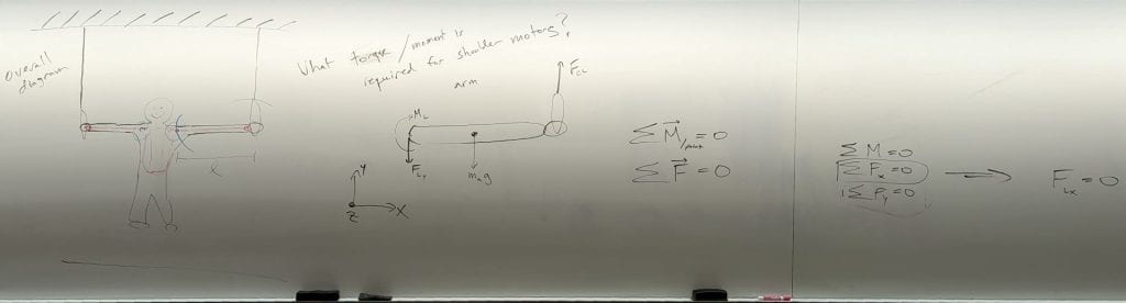
You can also download a PDF for the full robot-assisted iron-cross problem. We will finish this problem and go through other problems on the whiteboard during Friday’s lecture (8/26/2022).
8/26/2022 : Lecture 2 – Statics 2
I started by checking to make sure that students had access to the homework and understood that they should start right away, so that they can be fluent in time for the first homework quiz. We then spent the rest of the time working through problems that apply statics to biomedical engineering problems.
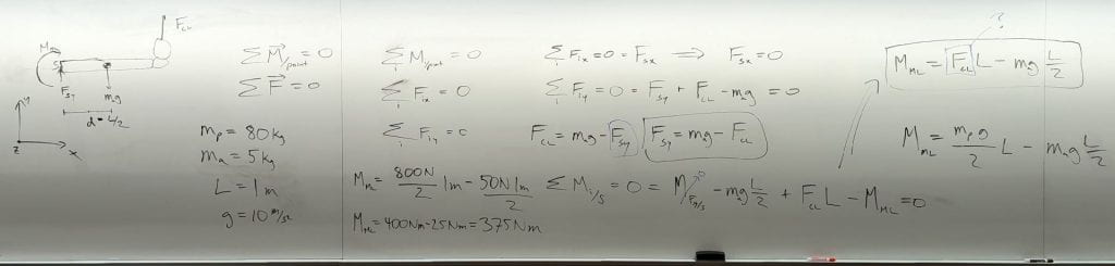
First, we worked through the remaining part of the robot-assisted iron-cross problem (PDF of the robot-assisted iron-cross problem). Notable aspects of our problem solving process include the following:
- For some forces and moments, we were confident about the direction and for others we were not. For example, we were confident about the direction of the force applied to the ring by the cable, and the direction of the gravitational force applied to the arm. In contrast, we were not confident about the direction of the vertical force applied to the arm’s pin joint at the shoulder.
- We used scalar forms of the static equilibrium equations. When we discovered that moments or forces were zero in our free-body diagrams (FBDs), we erased them. When we discovered that the direction of a force or moment was wrong in our FBD, we erased it and redrew it in the opposite direction.
- We carefully considered the variable for which we were solving, the variables with values we could estimate, and the variables with unknown values. This made us realize we needed to use a second FBD to find the force applied by the cable to the ring held by the hand of the arm. Later, considering the variables made us realize we needed a further assumption. We chose to assume bilateral symmetry, which implies that the left and right cable forces are equal due to the problem being the same when reflected across the midline of the person’s body.
- We made other approximations, including placing the arm’s center of mass in the middle of the arm, and using approximate low-precision values that are easy to work with, such as g=10m/s^2, and L=1m, so that we could more quickly arrive at an initial estimate.
- We discovered errors by checking the units of our answer. We also realized that we had neglected to include the gravitational force applied to the arm.

The iron-cross problem took most of the class. Students preferred working through problems slowly, which was also good for me, since it reduced the likelihood of confusing errors.
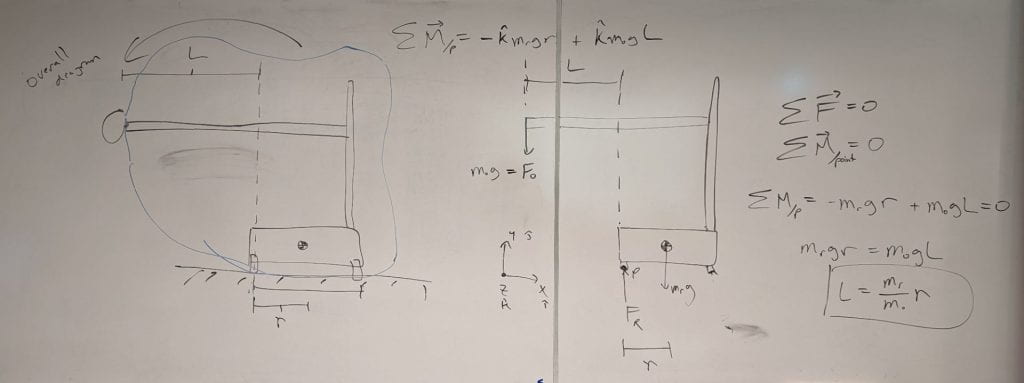
For the remainder of the class, we briefly worked on three problems. First, we went through a quick example of creating FBDs from an overall diagram of a person holding a weight by a cable. One of the main points was that cutting through a part results in equal and opposite loads applied to the two FBDs connected at the cut. When the two resulting parts are reconnected, the loads cancel each other out and disappear. So, cutting reveals the hidden internal loads. It’s also important not to draw a canceled load on an FBD.
You can download a PDF with a model of a person holding a weight suspended by a cable. A photo from the whiteboard follows.

We then went through the setup of a problem in which you press against your left arm using your right finger. This illustrates how we can sense the forces we’re applying, the forces being applied to us, and the internal moments through our skin, our muscles, and our body motion. For example, pressing on the proximal part of the left arm (e.g., the bicep) results in a smaller moment in the left shoulder than pressing on the distal part of the left arm (e.g., the left hand).
You can download a PDF with a model of pushing against your left arm with your right finger.
We then stood up and pressed down on our desks and lifted up on our desks while paying attention to the pressure on our palms and feet. We discussed the maximum downward force that they could apply to the desk, and the maximum upward force that they could apply. We also discussed how their feet felt as they varied the magnitude of the downward or upward force. Notably, their feet rocked forward or backwards due to the moment generated by the force applied by their palms. If we had time, we would have used a distributed load to model the pressure on their feet.
You can download a PDF with a model of pushing on a desk.
If we had additional time, we would have also gone through simple examples of using cross products to calculate moments.
8/29/2022 : Problem-Solving Studio on Statics (PSS 2)
For this PSS, we used the schedule we designed during our meta-PSS (PSS 1). We used rigid-body models in static equilibrium to solve the following two problems.
Robot Tipping Problem
Downloads: the problem and the solution
In PSS 1, the students asked for realism. The model in this problem helped with the invention, design, and commercialization of a device applicable to healthcare (see my conflict-of-interest statement below). Dr. Henry Clever and I invented the robot while we were both teaching BMED 3400 in the spring of 2017, so we wrote an exam problem about it. I used this model to help guide the design at the startup I co-founded, and it even ended up in a recent peer-reviewed publication about the robot. You can see an example of a person with severe impairments using the commercial research robot as an assistive device in his home in this Washington Post article.
- Several students misinterpreted the meaning of the constant L, resulting in more complicated equations. Carefully reading the problem should help avoid this type of error.
- You can use your own body as a model to gain intuition for the robot tipping problem. If you keep your feet next to each other and hold your arm out while someone pulls down on your arm, you can feel yourself tipping over. You might even notice that the magnitude of the force applied to one of your feet becomes lower. You can then separate your feet to increase the stability of your stance and perform the same action.
Human Handstand Problem
Downloads: the problem; solution part 1; and solution part 2
Prof. Frank Hammond wrote this excellent problem and generously gave me permission to share it here. It has a nice relationship to the robot tipping problem, since the person is maintaining their own stability while performing a handstand. The problem includes multiple masses, an articulated limb, and a distributed load.
- Students mistakenly used the constant describing the uniform distributed load in the equations for static equilibrium. Noticing that the constant has units of N/m can help avoid this error. The distributed load should first be converted to a concentrated load. By finding the center of pressure, the distributed load can be represented as a single force vector without a moment.

- Many students needed to lookup hip abduction and some misinterpreted the angle of hip abduction.
- Some students were confused by the squared term in the equations. This comes from the full length of the body (L) being used twice when computing the moment generated by the distributed load (M_breeze). Specifically, the magnitude of the concentrated force that represents the distributed load is F_breeze * L, and its moment arm with respect to a point at the hands is L/2.

How can you convince yourself that you’re right?
During the team problem solving segment, students would sometimes ask me if they had the correct answer. During quizzes, exams, and real-world problem solving, you need to find ways to convince yourself that you’re correct without the assurance of a higher authority. I attempted to help students find ways to check their own work. For example, they could use even simpler models to assess the plausibility of their answers. They could also assess the plausibility of their resulting equations by seeing what happens if an input parameter was doubled, halved, or set to zero.
Conflict of Interest Statement: In addition to being an associate professor at Georgia Tech, I am a co-founder and the chief technology officer (CTO) of Hello Robot Inc. where I work part time. I own equity in Hello Robot Inc. and I am an inventor of Georgia Tech intellectual property (IP) licensed by Hello Robot Inc. Consequently, I receive royalties through Georgia Tech for sales made by Hello Robot Inc. I also benefit from increases in the value of Hello Robot Inc.
8/31/2022 : Lecture 3 – Model of Simple Axial Loading 1
Assistive devices that give people greater independence can significantly enhance quality of life. In this lecture, we considered how to design a cable for a trapeze that people with mobility impairments can use to move themselves.
You can view my slides using Google Slides or by downloading a PDF of my slides. You can also download a PDF of the design problem and a vendor sheet for steel chain. We didn’t finish the problem in lecture and will briefly discuss it at the beginning of the next lecture.
For this design problem, a rigid body model fails to provide insight into key design decisions. For example, the choice of material strongly influences safety, yet an ideal rigid body doesn’t change shape or break regardless of the loads applied.
To address this, we began working with a deformable body model. Specifically, we started using a simple model of an elongated object to which an axial load has been applied. This enabled us to model how the cable’s material and cross-sectional area influence internal stress and lengthening.
When using the model, the sign convention for the scalar P often causes confusion. P > 0 implies that the object is in tension. P < 0 implies that the object is being compressed. The following whiteboard diagram may help.

As usual, we first drew an overall diagram and then isolated the cable.

We also discussed the importance of communicating the intended use of an engineered device. Communicating the intended use allows us to model the loads that the device will encounter when used properly and to include a margin of safety based on these expected loads.
9/2/2022 : Lecture 4 – Model of Simple Axial Loading 2
You can view my slides using Google Slides or by downloading a PDF of my slides. You can also download a final PDF on the trapeze design problem and two PDFs for the surgical design problem that complement the documentation below (PDF 1 and PDF 2).
Trapeze Design Problem Wrap Up
We wrapped up the trapeze design problem from the previous lecture by focusing on the minimum cross-sectional area we could use for different materials without the materials undergoing plastic deformation. You can download a PDF with the trapeze design problem wrap up and see the whiteboard photo below.

Surgical Robot Design Problem
Then we started a new design problem to evaluate a new material for use as a cable for a surgical robot. After the lecture, people expressed confusion with the problem. This is understandable, since we didn’t have much time to work on the problem. To help reduce confusion, I’ve used photos to document the solution here.
Before proceeding, please note that we use our simple axial loading model twice. First, we use it to model a cable for a surgical robot. Second, we use it to model a material sample.
First, we wanted to use our simple model of axial loading to estimate how much a cable made with the new material would lengthen when used in a surgical robot. So, we wanted to estimate δ, where δ=PL/AE. We quickly modeled the geometry for the cable with L_cable = 0.5 m and A_cable = 3×10^-6 m^2. We then estimated the load applied to the cable as P_cable = 40 N. You can find details in the problem PDFs (PDF 1 and PDF 2). At this point, we needed an estimate of Young’s modulus, E, for the new material. We had been given a sample of the new material, which we needed to use to estimate E.
Second, to estimate E for the material sample we were provided, we considered two approaches. We could use our model of simple axial loading to draw a stress-strain curve by plotting pairs of σ and ε (stress and strain) and then estimating the slope near the origin to find E. Or, we could directly use our simple axial loading model by rearranging the equation δ=PL/AE to be E=PL/Aδ and then finding P_sample, L_sample, A_sample, and δ_sample, which is the approach I will now illustrate.
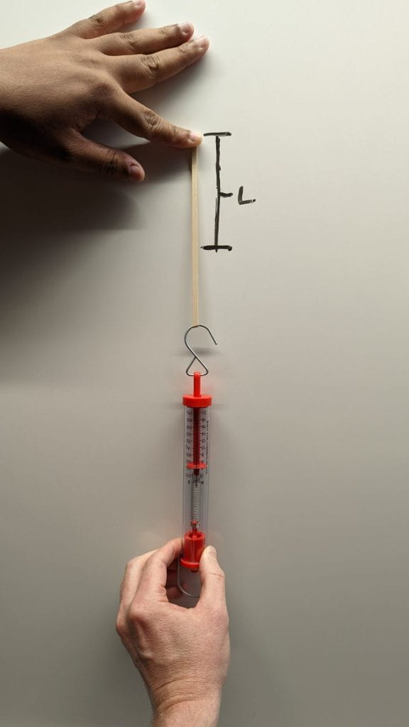
We can first measure L_sample by measuring the length of the unloaded material sample.

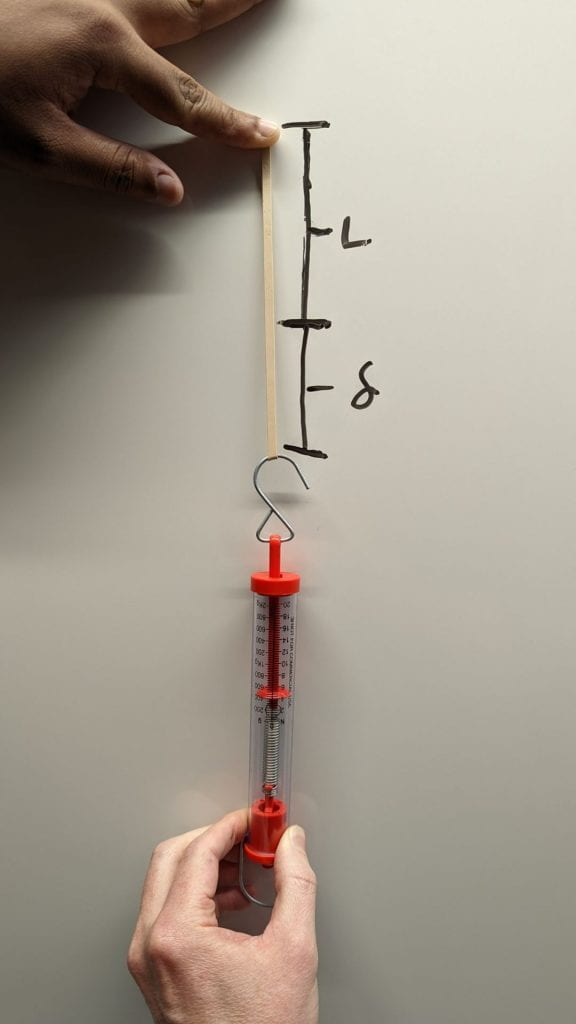
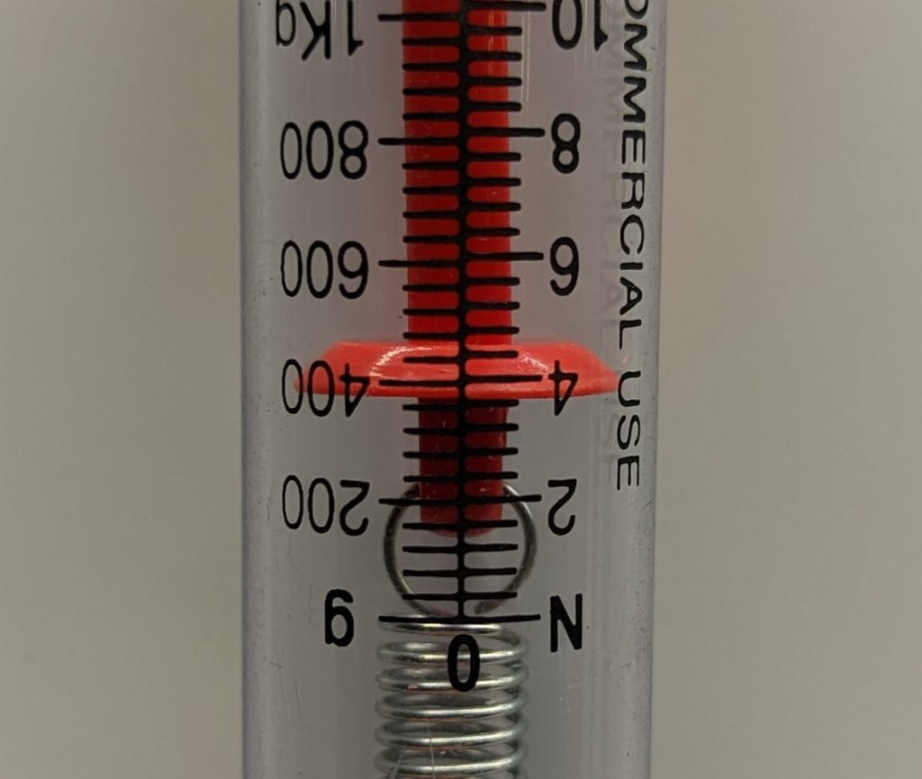
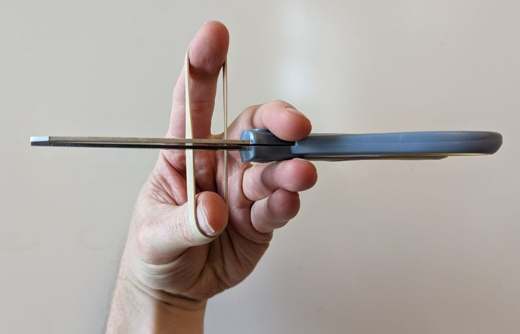
Then, we can apply a load and measure the change in length, δ_sample. We can use a spring scale to apply a known load, P_sample. For this step, a very kind person who stopped by the lecture hall after class helped by holding the top of the material sample while I applied a load. I’m grateful for his help, since I had been struggling to find a way to take a photo while doing it myself. Thank you James!
We now need to estimate the cross-sectional area for the material sample, A_sample, which we can do by cutting through it and measuring.
The cross-sectional area is composed of two rectangular cross sections with the same dimensions.
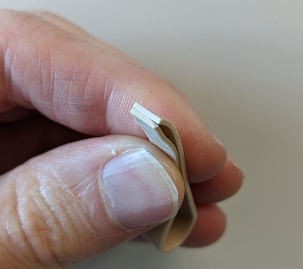
So, we measure the width and height of one of these rectangular cross sections.
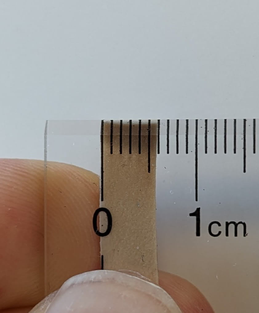

A single rectangular cross section has an area of approximately 6mm x 1mm = (6 x 10^-3m)(1 x 10^-3m) = 6 x 10^-6 m^2. So, the total cross-sectional area would be twice this, due to the two rectangular cross sections, giving us A_sample = 12 x 10^-6 m^2 = 1.2 x 10^-5 m^2.
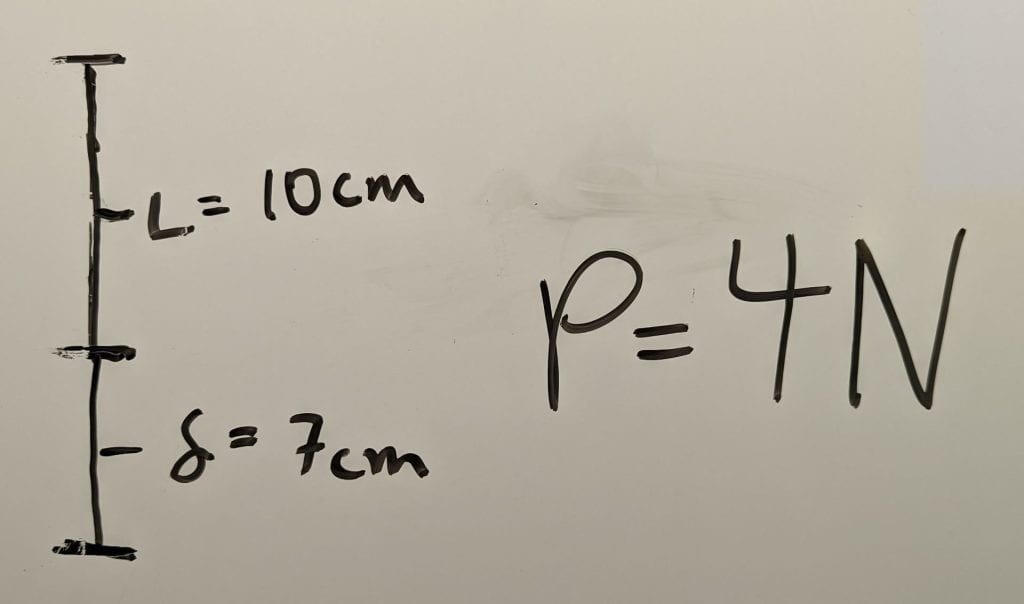
Putting this all together we obtain the following estimate for E_sample.
E_sample=(P_sample L_sample) / (A_sample δ_sample) = (4N * 1 x 10^-1 m) / (1.2 x 10^-5 m^2 * 7 x 10^-2 m) = (4 x 10^-1 Nm) / (8.4 x 10^-7 m^3) = 1/2.1 x 10^6 Pa ~= 0.5 MPa
So, we can estimate that E_sample = 0.5 MPa and then use this to calculate the expected elongation of a cable, δ_cable, used by a surgical robot made from the same material.
δ_cable = (P_cable L_cable) / (A_cable E) = (40 N * 0.5 m) / (3 x 10^-6 m^2 * 0.5 x 10^6 Pa) = 20 Nm / 1.5 N ~= 13 m.
Our model indicates that using the new material to fabricate a cable for a surgical robot is infeasible. Our model predicts that the cable would lengthen over 10 meters when gripping onto tissue during surgery! This is so far from being reasonable that our simple model will likely be sufficiently convincing. It also seems likely that the material would fail or plastically deform, since the total length would be 13.5 m = L_cable + δ_cable, which would be 27 times the original length of 0.5 m = L_cable!
9/7/2022 : Lecture 5 – Model of Axial Loading 1
We devoted the majority of the lecture period to Homework Quiz #1 [quiz][quiz solution]. Before the quiz, I introduced a more general model of axial loading for which quantities can vary along the length of the object [Google Slides][PDF of slides].
We started by observing a rubber band with evenly spaced markings as I applied a load to both ends. I then used scissors to reduce the cross-sectional area of the rubber band in the middle of its length, which resulted in the markings in the middle separating more when I applied a load. I then put an unaltered rubber band in series with a piece of plastic with much higher stiffness to observe that the rubber band lengthened much more than the plastic. Finally, I applied loads at the ends of a a rubber band and in the middle to show that with three local loads I could vary how much the top and bottom regions of the rubber band would lengthen.
After this demonstration, I gave an overview of the mathematical model as shown in our axial loading chart. I concluded by using low-order piecewise polynomials and graphs to apply this new axial loading model to the same situation we’ve analyzed with our simple axial loading model (see whiteboard photo). Both models predict the same total deformation, but the new model provides additional insight about how the cross sections of the object move, corresponding to the changes in the markings on the rubber band we observed [PDF with examples].

9/9/2022 : Lecture 6 – Model of Axial Loading 2
As usual, you can obtain my slides as Google Slides or a PDF. You can also download a PDF with the mathematical model used below.
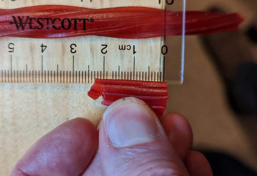
I started the lecture by describing my intentions when writing and administering quizzes and exams. After a brief review of our axial loading model, we started a catheter design problem. We used a Twizzler as a physical model of a catheter and a ruler to model the tissue as the catheter is pulled out. One person was responsible for modeling the tissue by holding the ruler on top of the Twizzler. Another person was responsible for modeling the healthcare worker pulling the catheter until it ruptured.
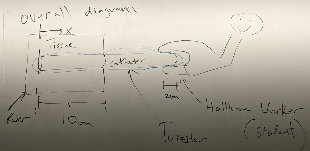
We set up the experiment so that people could pull until the Twizzler ruptured and then report where it failed. As shown in our overall diagram and the photos below, the ruler was placed over the first 10 cm of the Twizzler, and the class attendee held onto the last 2 cm of the Twizzler while pulling it until failure. Special thanks to Professor Melissa Kemp who pulled the Twizzler, while I held the ruler and took photos.
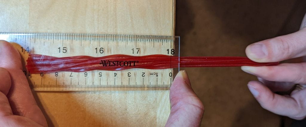
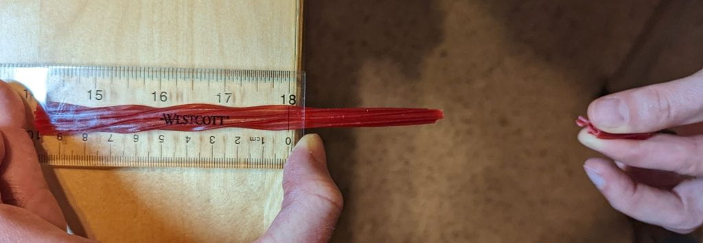
After pulling until failure, the team found the length at which the Twizzler failed, where 0 cm was at the end of the Twizzler under the ruler and 17 cm was at the end of the Twizzler held by the fingers.
We then created a histogram of the locations where the Twizzlers failed, which showed high numbers of failures just outside of the tissue model (ruler) or before the fingers. Each red X corresponds with a failure location reported by a person in the lecture.
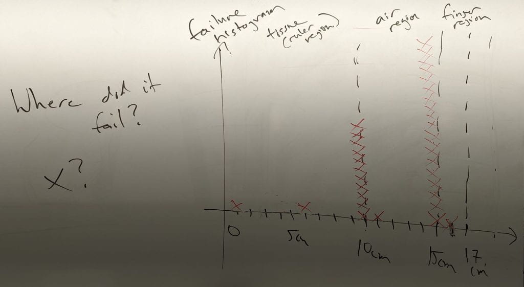
We then used a mathematical model, our axial loading model, to estimate where the normal stress was highest. You can see the region of maximal stress circled in red on the normal stress, σ(x), graph below. This region of maximal stress corresponds with the region of the Twizzler surrounded by air in our experiment. You can also download a PDF with a more careful and thorough model.
Unlike our simple axial loading model, which predicts the same stress everywhere, our axial loading model suggests that the stress would be highest in the air gap between the tissue and the fingers. This helps explain our empirical results, but doesn’t explain why the failures primarily happened near the boundaries of the tissue (ruler) and finger regions.

Professor Denis Tsygankov and the student he worked with during the class suggested that one might model the failure locations more precisely by varying the cross-sectional area, A(x). The ruler and fingers decrease the cross-sectional area by pushing down on the Twizzler to hold it in place and pull on it, respectively. Representing this decrease in area in and near the tissue and finger regions would lead to predictions of higher stress near the locations where the Twizzlers tended to fail. Prof. Tsygankov drew the following diagram after class to illustrate their idea.

9/12/2022 : Problem-Solving Studio on Axial Loading (PSS 3)
We worked through the following two problems.
- Distributed Load Problem (Solution) : This problem provides practice using our model of axial loading with a distributed load, constant Young’s modulus, and constant cross-sectional area. It asks for graphs of the key quantities. It does not apply the model to an application.
- Cancer Detection Problem (Solution 1, Solution 2) : This is an application focused problem that requires solving for deformation with varying material stiffness. The original solution used two simple axial loading models in series, but I wrote an additional solution that uses our model of axial loading with graphs to find the total deformation.
In this PSS, we focused on methods for efficient graphing of low-order piecewise polynomials. For example, calculating the areas of boxes and triangles provides key values for integrals of constant and linear functions.
We also looked at the function being integrated to find slopes for the resulting integral, since the function being integrated is the derivative of the result. This is useful for determining whether a linear function resulting from integrating a constant function should be increasing of decreasing. It’s also useful for finding the curvature of a quadratic function resulting from integrating a linear function, since the slopes at the beginning and end of the quadratic function determine whether it is concave up or concave down.
The whiteboard results for the first problem follow.

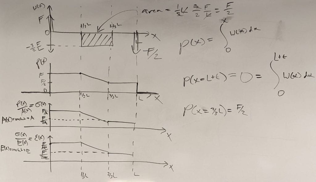
I also illustrated two simple examples that help me remember the sign convention for the applied distributed load, ω(x). These are helpful once you remember that the internal axial load, P(x), is positive for slivers that are in tension and negative for slivers that are in compression.

9/14/2022 : Lecture 7 – Model of Axial Loading 3
I only worked at the whiteboard, so I don’t have any slides to share. The following PDFs have my notes for the lecture.
- Representing a concentrated load with a Dirac delta function
- Example of graphs for axial loading with both compression and tension
- Two examples of axial loading graphs, one with varying Young’s modulus and the other with varying cross-sectional area
Representing a Concentrated Load as a Distributed Load
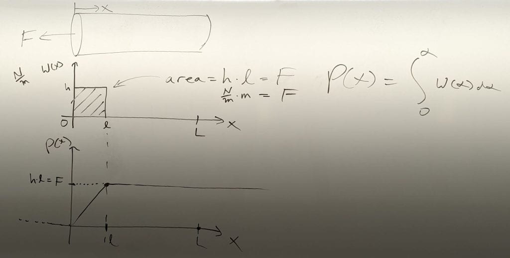
First, we discussed how we could create increasingly better approximations of a concentrated load of F Newtons using a box function distributed load with the area of F. The narrower and taller the box function, the better approximation. From this perspective, the Dirac delta function represents the absurd limit when the box has infinite height and infinitesimal width. By using a Dirac delta function, we get an excellent representation of a concentrated load and also simplify our calculations, since we don’t have the complexities of a linear function when we integrate.

Tension and Compression in the Same Object
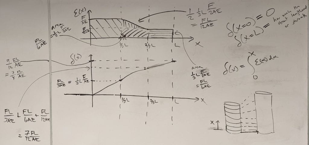
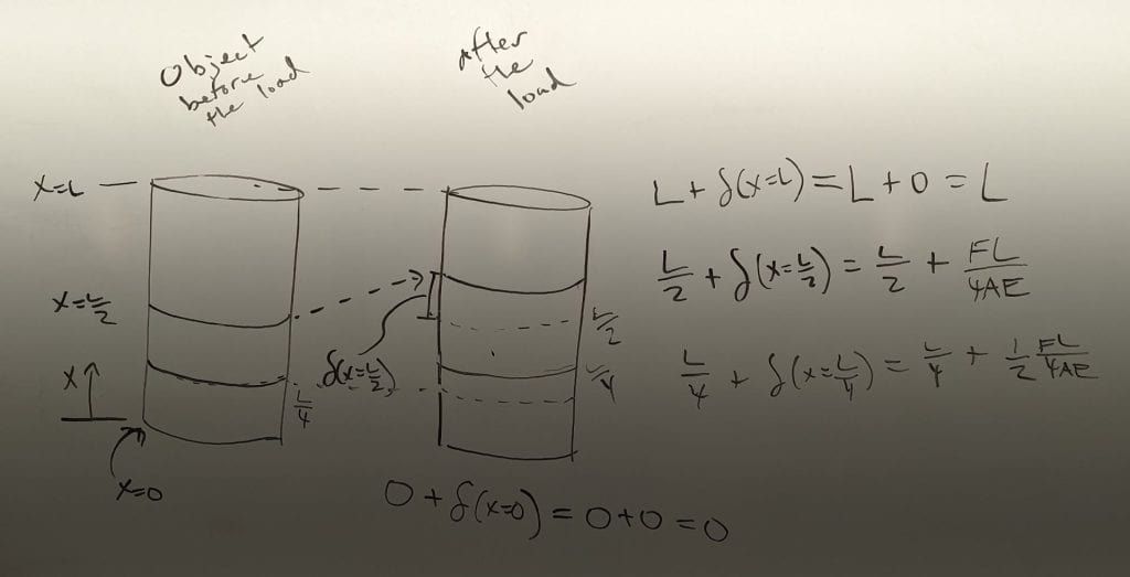
Next, we considered an example of an axially loaded object that has a region in tension, a region in compression, and a total deformation of zero.

We paid close attention to the signs of the various functions of x associated with our axial loading model. Notably, the internal axial load P(x), stress σ(x), and strain ε(x) are positive when the sliver at x is in tension and negative when the sliver at x is in compression. This is true for P(x) due to our sign convention. σ(x)=P(x)/A(x), so it follows the same sign convention since the cross-sectional area A(x)>0. ε(x)=σ(x)/E(x), so it follows the same sign convention when E(x) > 0, which is true for almost all materials. Apparently, there are rare exotic materials that can be modeled as having a negative Young’s modulus, but you are unlikely to encounter them and the applicability of our axial loading model is unclear.
We solved for the deformation function, δ(x), by drawing a series of graphs. Then we spent time interpreting the meaning of δ(x), which represents how far the cross section at x moved. Notably, for this problem both the cross section at x=0 and the cross section at x=L do not move, so δ(x=0)=0 and δ(x=L)=0.
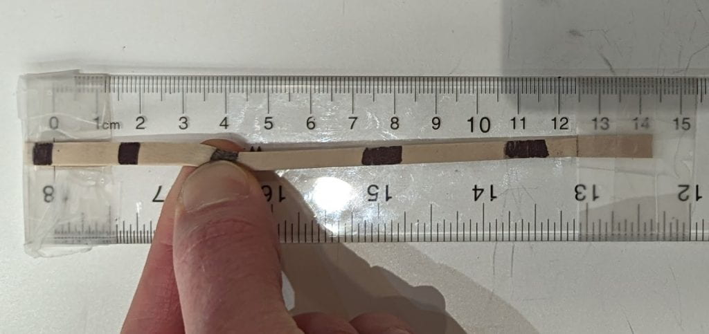
We then considered a similar physical model. I taped the ends of a rubber band onto a ruler and made evenly spaced markings along its length.

The deformation matched what we expected from our model. When loaded, the markings were closer together in the compressed region and farther apart in the tensile region. Also, when loaded, the markings in the compressed region were evenly spaced and the markings in the tensile region were evenly spaced. For example, the marking in the middle of the unloaded tensile region remained in the middle of the tensile region after loading. Likewise, the marking in the middle of the unloaded compressed region remained in the middle of the compressed region after loading. This corresponds with the linear regions of the deformation function, δ(x).
Varying Cross-sectional Area
We quickly went through the initial graphs for an object with varying cross-sectional area. The important thing is to be careful when graphing the stress σ(x) and strain ε(x). The stress σ(x) depends on the cross-sectional area, A(x), and the strain ε(x) depends on Young’s modulus, E(x). If A(x) or E(x) is not constant, your graphs need to represent this.

9/16/2022 : Lecture 8 – Statically Indeterminate Systems 1
We devoted the majority of the lecture period to Homework Quiz #2 [quiz][quiz solution].
With the remaining 15 minutes, I introduced static indeterminacy through an example problem [first problem in this PDF]. You can obtain my slides as Google Slides or a PDF.
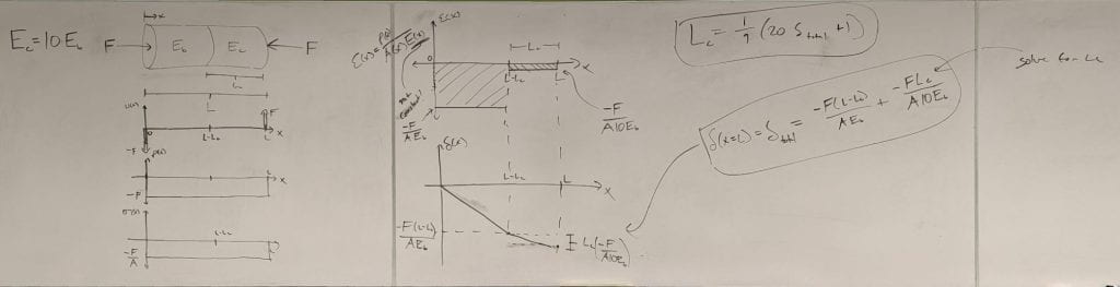
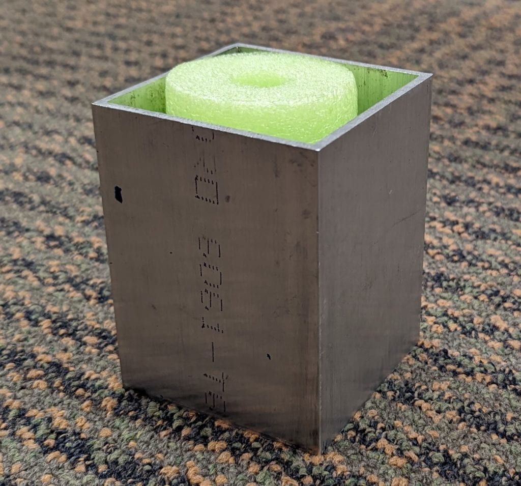
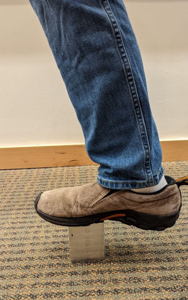
For the example problem, I included a physical demonstration consisting of an extruded aluminum tube with a foam tube placed inside of it. Our goal was to model what would happen if I stepped on this object consisting of two materials in parallel with very different values for Young’s modulus.

9/19/2022 : Problem-Solving Studio on Axial Loading (PSS 4)
- Young’s Modulus for Materials [problem][solution]: It’s valuable to have intuition for the stiffness of materials that are used in biomedical engineering. This problem involves sorting materials into three coarse categories (GPa, MPa, kPa) separated by three orders of magnitude.
- Deformed Regions [problem][solution]: This problem helps reinforce how geometries change given an axial load and the sign conventions used by our model.
- Microneedle Problem [problem][solution]: This is a realistic problem that involves a varying cross section. A solution can be found more easily than you might at first imagine.
9/21/2022 : Lecture 9 – Statically Indeterminate Systems 2
You can download the slides [Google Slides][PDF] and lecture notes [PDF 1][PDF 2][PDF 3].
9/23/2022 : Lecture 10 – Review for Exam #1
You can download the slides [Google Slides][PDF].
9/26/2022 : Problem-Solving Studio on Statically Indeterminate Systems (PSS 5)
- Statically Indeterminate [problem][solution]: This is a short problem that provides examples of assumptions that can be made to resolve statically indeterminate systems.
- Linear System [problem][solution]: This is another short problem that should help clarify superposition, which I only discussed briefly at the end of Wednesday’s lecture. I consider it an important concept worth revisiting.
- Insole Design [problem][solution]: This is a realistic problem that involves splitting the cross-sectional area of an axially loaded object into a mix of two materials. The goal is to create an object that behaves similarly to an object made of a third material with Young’s modulus in between the original two materials.
The End!
My third of the class ends with Exam #1. Prof. Scott Hollister will be leading the next third, and Prof. Denis Tsygankov will lead the last third.